Lab 9: Mapping

Orientation Control

I chose orientation control because it was the offered a good balance between reliability and ease-of-implementation. To ensure yaw measurement accuracy, I used the onboard DMP chip by following Stephen Wagner’s tutorial on the course website. Essentially, the DMP combines gyroscope and accelerometer readings to calculate yaw without drift. To issue with the DMP calculation is that when yaw increases past 180, it wraps around to -180 and continues to increase from there. The wrap-around happens in the opposite direction when decreasing past -180. This behavior breaks my current implementation of the rotational PID controller. To fix this issue, I scan for wraparounds and add or subtract 360 depending on the direction.

// yaw calculation from DMP
double yaw = atan2(t3, t4) * 180.0 / PI;

// find difference between measurements
double yaw_diff = yaw - previous_yaw;
//_-360 depending on direction
if (yaw_diff > 180.0) {
    yaw_diff -= 360.0;
} else if (yaw_diff < -180.0) {
    yaw_diff += 360.0;
}
// accumulated_yaw has the same behavior as the normal gyro
accumulated_yaw += yaw_diff;
previous_yaw = yaw;

I decided to rotate my robot at 5 degrees increments, which gives 72 orientations for a full rotation. For each orientation step, I allow an error bound of 3 degrees and change the set-point to the current orientation plus 5 degrees. The challenge with using PID for these small incremental changes is that overshoot will result in bad TOF measurements. My solution for this was to increment the rotational deadband from 40 to 60, and setting the PID parameters to Kp = 0.1, Ki = 0, and Kd = 0. The mapping code is placed in the main loop()and is activated using the START_MAPPING BLE command.

currTime = millis();
// PID calculation 
float pid = motorController.compute(accumulated_yaw, currTime);

if(abs(motorController.getSetpoint() - accumulated_yaw) > 3){
    // change motor values if not within error bound
    motorDriver.handleTurningPID(pid);
}else{
    // otherwise, stop motors and update setpoint
    motorDriver.stopMotors();
    setPoint = accumulated_yaw + 5;
    motorController.setSetpoint(setPoint);
    pid = 0;
}

For this reason, I have high confidence in my yaw values. Sadly, the robot can’t stay on the same axis throughout the entire rotation. Over the course of collecting data, I found that the robot strays from its starting point by an average of 1 inch and a maximum of 2 inches. In a 4m x 4m square, this means an average error of 0.0635% and a maximum error of 0.127%. The video below shows the robot pivoting incrementally.

Read out Distances

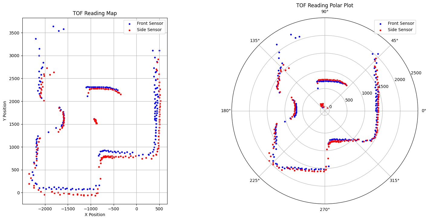
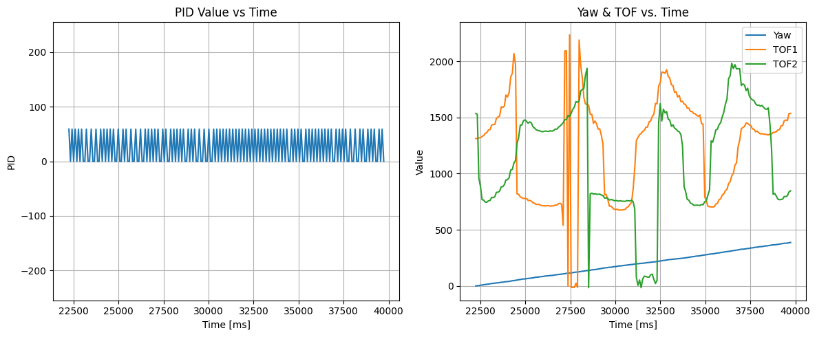
I executed the orientation control at the marked positions in the world space ((-3,-2), (5,3), (0,0), (0,3), and (5,-3)). During the turns I collected distance data from the two TOF sensors on my robot, one positioned at the front and the other at the side. I also kept track of time, PID values, and yaw. Upon making a full rotation, the robot stops and sends the relevant data arrays to my computer using BLE. In the next part of the lab, I will need to merge and plot the readings at each point, so it was important that the robot starts at the same orientation in all scans. The DMP calculated angle is saved at each step, NOT the set-point. I think of the PID system as leading a pig (DMP yaw) with a carrot (set-point). We are interested in the position of the pig, not the carrot. Since there is an error bound of 3-degrees, the TOF reading might not be evenly spaced, but at least they will be accurate. Shown below are mappings generated by the individual scans. Additionally, I included PID values over time and TOF readings over time. On the PID data, since Kp is so small, the values basically toggle between 0, and 60. This is a good because it means each rotational step is consistent and doesn’t overshoot. Rotating twice or more generates the same mapping, but with more granular data points. This means that the scans are precise and reliable.

(0,0):

(5,3):

(5,-3):

(0,3):

(-2,-3):

For the plots shown above, the front and side sensor readings have already been merged to the rectangular plane. I will talk about how I did this in the next section. It is important to notice that there is some discrepancy between the front and side sensor readings. Specifically, the side sensor gets blocked by the ground and the wheels more often than the front sensor. This makes sense because the front sensor is in a more exposed position. Because of this, I will be using the front sensor plots to create my final merged plot.

Merge and Plot Readings

To merge and plot the measurement data, I need a rotation and translation matrixes. The rotation matrix maps the polar coordinates onto a rectangular plane, with the center of the car as the origin. The translational matrix moves the readings from each of the sampling positions onto the same references frame, so all the individual maps line up to create a merged map. Since both sensors are not placed at the center of the car, I needed separate matrices to keep track of the sensor positions at each scanning position.

# (0,0)
frontSensorPos = np.array([[75], [0]])
sideSensorPos = np.array([[0], [40]])
# (5,-3)
frontSensorPos = np.array([[-304.8 * 3], [304.8 * 5 + 75]])
sideSensorPos = np.array([[40 - 304.8 * 3], [304.8 * 5]])
# (5,3)
frontSensorPos = np.array([[304.8 * 3], [304.8 * 5 + 75]])
sideSensorPos = np.array([[40 + 304.8 * 3], [304.8 * 5]])
# (0,3)
frontSensorPos = np.array([[304.8 * 3], [75]])
sideSensorPos = np.array([[40 + 304.8 * 3], [0]])
# (-2,-3)
frontSensorPos = np.array([[-304.8 * 2], [-304.8 * 3 + 75]])
sideSensorPos = np.array([[40 - 304.8 * 2], [-304.8 * 3]])

The origin matrix is the most understandable, and it tells us the the front sensor is 75mm from the center of the robot, while the side sensor is 40mm from the center of the robot. The rotational matrix is dependent on the angle (yaw) or each measurement, and is shown below:

def rMatrix(yaw):
    # convert to radians
    radYaw = np.radians(yaw)
    return np.array([[np.cos(radYaw), np.sin(radYaw)],
        [np.sin(radYaw), -np.cos(radYaw)]])

Similar to how Ming He (Spring 2024) did it in his lab report, I applied the rotation and translation matrices to the my recorded data using a for-loop.

for angle, frontDist, sideDist in zip(yawArr, tof1Arr, tof2Arr):
    # calculate rotation matrix
    rotationMatrix = rMatrix(angle)
    # transform front sensor data
    frontPoint = np.matmul(rotationMatrix, 
        np.array([[frontDist],[0]])) + frontSensorPos
    # transform side sensor data
    sidePoint = np.matmul(rotationMatrix, 
        np.array([[0],[sideDist]])) + sideSensorPos
    # add to transformed points
    frontTransformed.append(frontPoint)
    sideTransformed.append(sidePoint)

Using this code, I was able to merge and plot all of the readings from the various positions onto one graph, shown below:

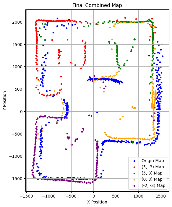
Visually speaking, the robot did a good job at mapping its environment.

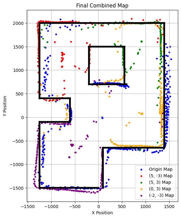
Convert to Line-Based Map

Finally, I needed to convert the merged map into a line-based map so that the simulator can use it. The lines were manually estimated and plotted on the same axes. For some reason, the robot missed the center part of the top portion of the inner square. This might be because the 5 degree increment was too big to capture certain details in the world. If I were to do these measurements again, I would decrease the increment from 5 to 3 and see if it improved the result. This was acceptable for this lab because it is easy to estimate where the top part should be.

# Outer Border
ax1.plot([-1250, 1400], [2000, 2000], 'k', linewidth = 4)
ax1.plot([-1250, -1250], [400, 2000], 'k', linewidth = 4)
ax1.plot([-1250, -600], [400, 400], 'k', linewidth = 4)
ax1.plot([-600, -600], [400, -100], 'k', linewidth = 4)
ax1.plot([-600, -1250], [-100, -100], 'k', linewidth = 4)
ax1.plot([-1250, -1250], [-1500, -100], 'k', linewidth = 4)
ax1.plot([-1250, 0], [-1500, -1500], 'k', linewidth = 4)
ax1.plot([100, 100], [-650, -1500], 'k', linewidth = 4)
ax1.plot([100, 1400], [-650, -650], 'k', linewidth = 4)
ax1.plot([1400, 1400], [-650, 2000], 'k', linewidth = 4)

# Inner Square
ax1.plot([-200, 600], [700, 700], 'k', linewidth = 4)
ax1.plot([-200, -200], [700, 1500], 'k', linewidth = 4)
ax1.plot([-200, 550], [1500, 1500], 'k', linewidth = 4)
ax1.plot([550, 550], [1500, 700], 'k', linewidth = 4)

References

• Mikayla Lahr Course Webpage: for getting a better idea of what graphs and information were needed
• Ming He Lab 9 Report: referenced for how to design transformation matrices and using for-loop to apply then to the data
• Stephen Wagner Lab 6 and Lab 9 Report and DMP Tutorial: super helpful for getting rid of sensor drift and ensuring accuracy
• Professor Helbing and TAs during open hours: Thanks for helping me solve the issue with the DMP where the FIFO wasn’t clearing!