Lab 7: Kalman Filtering

In this lab, I will implement a Kalman filter to enhance the performance of the robot while approaching walls. A Kalman filter has two stages, prediction and correction. In the prediction stage, it uses a state-space model to predict the current state based on previous states and inputs. In the correction stage, it weighs the uncertainty between the model and actual readings to refine the prediction. The Kalman filter will overcome the limitations imposed by the slow ToF sensors, allowing the robot to approach walls at higher speeds while maintaining the ability to either stop 1 ft from the wall or execute a turn within 2 feet.

Estimate Drag and Momentum

Before I can define my state-space equations and solve for the $A$ and $B$ matrices, I need to find drag and momentum. To do this, I created a new Bluetooth command that:

1. Initializes arrays to hold transmission data
2. Keeps track of time, motor input, and distance from wall
3. Steps up the motor input while sampling
4. Transmits the array data over Bluetooth

These variations of these functions have been extensively covered in previous labs (especially lab 5), so I will not include code for this command. For my step response, I chose 150, which is ~60% of the maximum speed achieved in the lab 5 PID system (255). Using the distance over time data, I calculated the forward velocity using np.gradient().

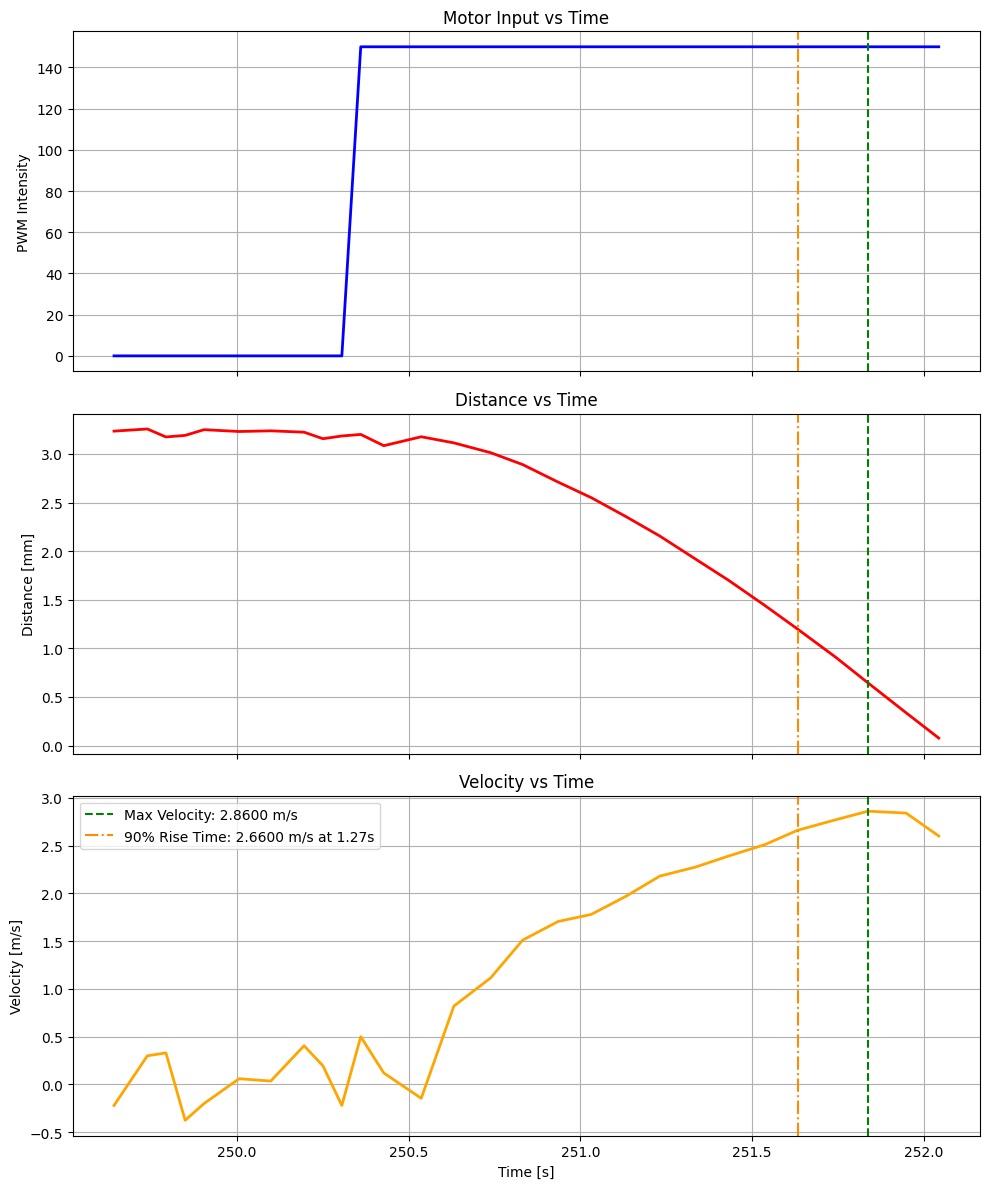
From the step response graph, we can see that:

• The maximum forward velocity is 2.86 m/s, so we can assume that it would plateau there if the motor were to continue running.
• The speed at 90% rise time is $0.90 \times 2.86 = 2.66 \text{ m/s}$
• The 90% rise time is 1.27s

Using this numbers, I can estimate drag and momentum. Drag is the magnitude of the step response divided by the steady state speed.

\[d = \frac{u}{\dot x} = \frac{1}{2860} = 0.000350\]

Momentum can be solved using this equation.

\[m = \frac{-d \times t}{\ln(0.1)} = \frac{-0.000350 \times 1.27}{\ln(0.1)} = 0.000193\]

Initialize Kalman Filter

The equations for $A$ and $B$ are shown below:

\[A = \begin{bmatrix} 0 & 1 \\ 0 & \frac{d}{m} \end{bmatrix}\] \[B = \begin{bmatrix} 1 \\ \frac{1}{m} \end{bmatrix}\]

Since we already known $d$ and $m$, solving for $A$ and $B$ is simply plug-and-chug:

\[A = \begin{bmatrix} 0 & 1 \\ 0 & 1.8112 \end{bmatrix}\] \[B = \begin{bmatrix} 1 \\ 5180.1689 \end{bmatrix}\]

Then, I discretized my matrices using the loop frequency that I found in lab 5 (300 Hz).

\[A_d = I + A \cdot dt = \begin{bmatrix} 1 & 0 \\ 0 & 1 \end{bmatrix} + \begin{bmatrix} 0 & 1 \\ 0 & 1.8112 \end{bmatrix} * dt = \begin{bmatrix} 1 & 0.0033 \\ 0 & 0.9940 \end{bmatrix}\] \[B_d = B \cdot dt = \begin{bmatrix} 1 \\ 5180.1689 \end{bmatrix} * dt = \begin{bmatrix} 1 \\ 17.2712 \end{bmatrix}\]

The C matrix is show below, where the top term is distance and the bottom term is velocity.

\[C = \begin{bmatrix} 1 \\ 17.2712 \end{bmatrix}\]

I also needed to specify process and sensor noise covariance to create the process noise matrix.

\[\sigma_1 = \sqrt{10^2 \times \frac{1}{0.10}} = 31.62\] \[\sigma_2 = \sqrt{10^2 \times \frac{1}{0.10}} = 31.62\] \[\Sigma_u = \begin{bmatrix} \sigma_1^2 & 0 \\ 0 & \sigma_2^2 \end{bmatrix} = \begin{bmatrix} 1000 & 0 \\ 0 & 1000 \end{bmatrix}\]

According to the lecture slides, the measurement noise is equation to the long distance ranging error.

\[\sigma_3 = 20\]

Implement Kalman Filter in Jupyter

The code shown below is a python implementation of the calculations from the last section. There are several variables that can be modified to tune to system.

# drag and momentum
d = 0.000350
m = 0.000193

# A and B matrices
A = np.array([[0, 1], [0, -(d / m)]])
B = np.array([[0], [1 / m]])

# frequency and time step
freq = 300
dt = 1 / freq

# discretized A and B, C matrix
Ad = np.eye(2) + (A * dt)
Bd = B * dt
C = np.array([[1, 0]])  

# sampling frequency
tofFreq = 10

# process and measurement noise
sigma_x = np.sqrt(100 * tofFreq)
sigma_dx = np.sqrt(100 * tofFreq)
sigma_noise = 20

# noise matrices
Sigma_u = np.array([[sigma_x**2, 0], [0, sigma_dx**2]])
Sigma_z = np.array([[sigma_noise**2]])
Sigma_init = np.array([[20**2, 0], [0, 1**2]])

With the calculations finished, I used the Kalman filter function provided in the lab manual:

def kf(mu, sigma, u, y):
    mu_p = Ad.dot(mu) + Bd.dot(u) 
    sigma_p = Ad.dot(sigma.dot(Ad.transpose())) + Sigma_u
    K = sigma_p.dot(C.transpose().dot(np.linalg.inv(C.dot(sigma_p.dot(C.transpose())) + Sigma_z)))
    y_m = y - C.dot(mu_p)
    mu = mu_p + K.dot(y_m)    
    sigma = (np.eye(2) - K.dot(C)).dot(sigma_p)
    return mu, sigma

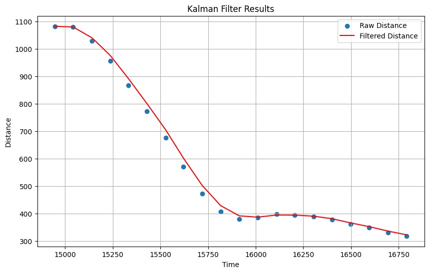
I ran the Kalman filter on the step response data and graphed the result.

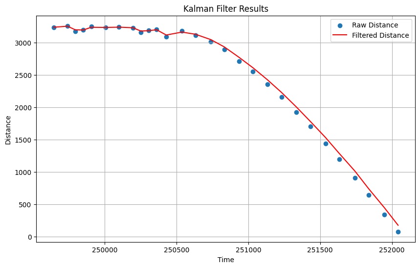
The graph shows that the filter slightly over-fits the data when the distance delta is small and slightly lags the data when the distance delta is larger. Overall, the filter is acceptable, so I decided to stick with these values for now. If I want to decrease over-fitting in at low deltas, I can increase the measurement noise variance ($\sigma_m$), but it comes at the cost increasing lag at high deltas.

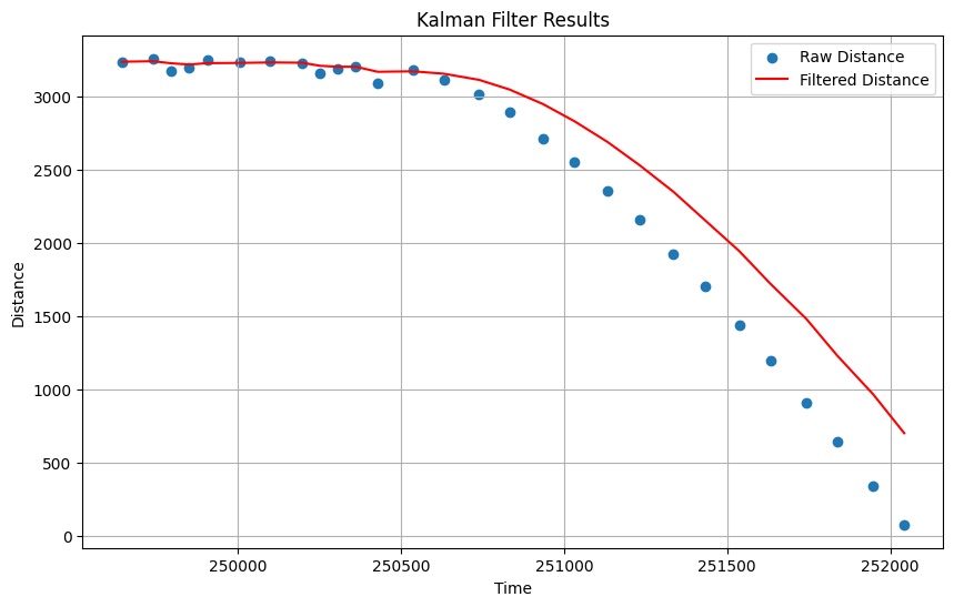
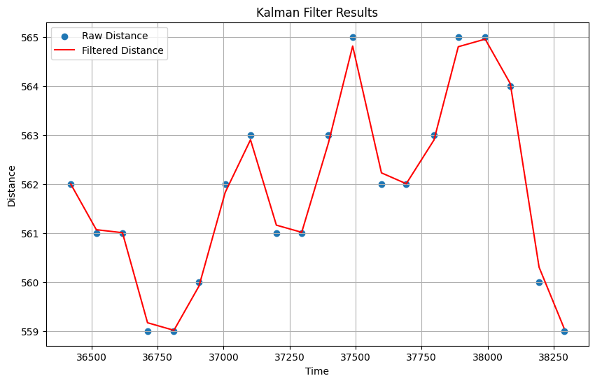
This result is not desirable, so I decided to decrease process noise variance ($\sigma_p$), giving the result shown below:

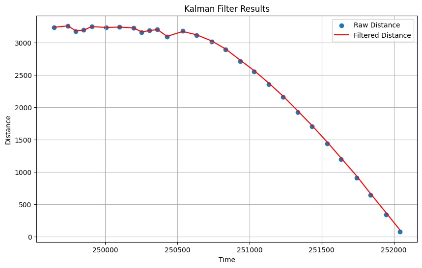
The data is clearly overfitted, so I decided to stick with my initial calculated values, which was a good compromise between overfitting and lag, minimizing both. To test my Kalman filter, I chose a lab 5 run where my robot over-braked from the derivative portion of the PID controller, and then settled into the equilibrium setpoint. This data shows that the Kalman filter has the flexibility to deal with unconventional movements, while not over-fitting to the data.

Implement Kalman Filter on Robot

Since the Kalman filter is state-based, I decided to implement my Kalman filter using a class. The constructor KalmanFilter() uses the drag, momentum, and loop time values to initialize and discretize the matrices, shown below:

KalmanFilter::KalmanFilter(){
  // filter has not received first reading yet
  _initialized = false;

  // set drag and momentum
  float d = 0.000350;
  float m = 0.000193;

  // declare A, B, C and I matrices
  BLA::Matrix<2, 2> A = { 0, 1, 0, -d / m };
  BLA::Matrix<2, 1> B = { 0, 1 / m };
  C = {1 , 0};
  I = {1, 0, 0, 1};

  // time step
  _dt = 0.0033;

  // discretize A and B
  Ad = I + ( A * dt );
  Bd = B * dt;

  // error fields
  _sigU = {1000, 0, 0, 1000};
  _sigN = 20;
  _sigZ = {_sigN * _sigN};
  _sigma = {_sigN * _sigN, 0, 0, 1};
}

Using this setup, I created an update() function that is a duplicate of the Jupyter logic shown in the previous section. However, I found it difficult to calculate the filtered values in between readings without rewriting the entire implementation, so the filter just generates values that are offset from reality and didn’t have positive effects on the speed or accuracy of the PID system.

References

• Nidhi Sonwalker Course Webpage for clarification on matrix calculations
• Consulted Ben Liao for understanding what makes a Kalman filter good