Lab 6: Orientation PID Control
This lab focuses on achieving stationary orientation control using a PID controller. When the orientation of the robot is perturbed, the wheels should spin in opposite directions at the same speed to rotate the robot back to the set point.
Prelab
Testing the PID controller for this lab will be faster than than lab 5. The robot remains stationary, so there is no need to reposition the robot after every test. Therefore, tuning the PID gains quickly will be essential. Additionally, I want to be able to change the robot setpoint using BLE commands while the PID loop is running. Since my lab 5 PID loop lives inside of a BLE command, I can’t send new commands while it is running. For this lab, I moved my PID controller to the Arduino loop function. This way, the BLEUpdate function is called after each iteration of PID calculation to check for new commands.
1
2
3
4
5
6
while (central.connected()) {
    BLEUpdate();
    if(activePID){
        // calculate PID output and change motor PWM
    }
}
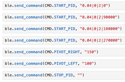
The controller starts when I send the START_PID command, which toggles the global variable activePID from 0 to 1 and sets the PID gains. Conversely, sending the STOP_PID command will toggle activePID from 1 to 0, stopping the PID controller, without changing the PID gains.
1
2
3
4
5
6
7
8
9
10
11
12
13
14
15
16
17
18
19
20
case START_PID:
    // set PID to active
    activePID = 1;
    // recieve kp,i,d from BLE
    success = robot_cmd.get_next_value(kp);
    if(!success){return;}
    success = robot_cmd.get_next_value(ki);
    if(!success){return;}
    success = robot_cmd.get_next_value(kd);
    if(!success){return;}
    success = robot_cmd.get_next_value(targetYaw);
    if(!success){return;}
    break;

case STOP_PID:
    // set PID to inactive
    activePID = 0;
    i = 0;
    stopMotors();
    break;
I will need to graph the set point, yaw angle, and motor input.I made few modifications to my SEND_PID_DATA command from lab 5 to support this.
1
2
3
4
5
6
7
8
9
10
11
12
13
14
15
16
17
case SEND_PID_DATA:
    Serial.println("Sending PID Data");
    for(int j = 1; j < MAX_SAMPLES; j++){
        tx_estring_value.clear();
        tx_estring_value.append(timeData[j]);
        tx_estring_value.append(" ");
        tx_estring_value.append(yawData[j]);
        tx_estring_value.append(" ");
        tx_estring_value.append((int)PIDData[j]);
        tx_estring_value.append(" ");
        tx_estring_value.append(setPointData[j]);
        tx_characteristic_string.writeValue(tx_estring_value.c_str());
        Serial.println(tx_estring_value.c_str());
        tx_estring_value.clear();
    }
    Serial.println("Done Sending PID Data!");
    break;
I also made a couple of changes to my notification handler. Specifically, I changed the name of the arrays that save data and the amount of data arrays that are filled out.
1
2
3
4
5
6
7
8
9
10
11
12
13
14
15
def notif_handler(uuid, byte_array):
    msg = ble.bytearray_to_string(byte_array)
    data = msg.split(" ");
    for i in range(4):
        if(i == 0):
            time_arr.append(int(data[i]))
        elif(i == 1):
            yaw_arr.append(float(data[i]))
        elif(i == 2):
            pid_arr.append(float(data[i]))
        elif(i == 3):
            set_point_arr.append(float(data[i]))
    print("Data Received")

ble.start_notify(ble.uuid['RX_STRING'], notif_handler)
I made some adjustments to the graphing script as well.
1
2
3
4
5
6
7
8
9
10
11
12
13
14
15
16
17
18
19
20
21
22
23
24
25
26
27
28
29
30
31
32
33
34
35
36
37
38
import matplotlib.pyplot as plt
fig, axs = plt.subplots(3, 1, figsize=(10, 12), sharex=True)
fig.subplots_adjust(hspace=0.3)  # Add some space between subplots


# Plot 2: Set Point
axs[0].plot(time_arr, set_point_arr, color='orange', linewidth=2)
axs[0].set_title('Set Point vs Time')
axs[0].set_ylabel('Set Point [mDeg]')

axs[0].grid(True)

# Plot 1: Yaw
axs[1].plot(time_arr, yaw_arr, color='blue', linewidth=2)
axs[1].set_title('Yaw vs Time')
axs[1].set_ylabel('Yaw [mDeg]')
axs[1].grid(True)

# Plot 2: PID
axs[2].plot(time_arr, pid_arr, color='red', linewidth=2)
axs[2].set_title('PID vs Time')
axs[2].set_ylabel('Intensity')
axs[2].set_xlabel('Time [ms]')
axs[2].grid(True)


fig.suptitle('Kp = 0.040, Ki = 0.000, Kd = 2.000', fontsize=16)
plt.tight_layout(rect=[0, 0, 1, 0.97])
plt.show()

plt.plot(time_arr[0:100], rawDist_arr[0:100], label = "Raw Data")
plt.plot(time_arr[0:100], dist_arr[0:100], label = "Extrapolated Data")
plt.title("Raw vs. Extrapolated Distance Data")
plt.xlabel("Time [ms]")
plt.ylabel("Distance [mm]")
plt.grid()
plt.legend()
plt.show()
Here are some jupyter cells that I used to test and debug the system.
Lab Questions:
PID Input Signal
Are there any problems that digital integration might lead to over time? Are there ways to minimize these problems?
The fundamental problem with gyroscopes is that, even at rest, they output small non-zero values. This could be caused by small vibrations, electrical noise, or even temperature. When I integrate the gyroscope to calculate orientation, each tiny error gets added to the next calculation. This causes the error to accumulate and compound over time. There are several ways to minimize these problems. The linear forces felt by the accelerometer can mathematically translated into rotational information, which can be used to stabilize the gyroscope. Alternatively, the magnetometer could be used to establish an absolute heading reference, since the Earth’s magnetic field doesn’t drift over time.
Does your sensor have any bias, and are there ways to fix this? How fast does your error grow as a result of this bias?
My sensor has bias, but it is not enough to cause issues in the short term. I found that placing my robot on a hard surface greatly reduced the bias of gyroscope. From previous labs, I found that my error grows at a rate of about 1 degree per second. I could have used the digital motion processor (DMP) to fix this error, but after comparing drift rates with some classmates, I determined that my drift rate is too slow to warrant the DMP, at least for this lab.
Are there limitations on the sensor itself to be aware of? What is the maximum rotational velocity that the gyroscope can read (look at spec sheets and code documentation on github). Is this sufficient for our applications, and is there was to configure this parameter?
The main limitation to be aware of is that the sensor has a default maximum spin rate of 250 degrees per second. Since my robot is able to complete a full spin in 700 ms, this default rate is not sufficient for the application. To configure this parameter, I referenced the IMU example code and increased the parameter to 500 degrees per second using the code shown below:
1
2
3
    ICM_20948_fss_t myFSS;
    myFSS.g = dps500;
    myICM.setFullScale((ICM_20948_Internal_Acc | ICM_20948_Internal_Gyr), myFSS);
The trade-off of increasing the sample rate is that each individual reading is less accurate, leading to faster drift. Nonetheless, 500 degrees per second still gave acceptable results for the purpose of this lab. I would be hesitant to increase the sample rate any more.
Derivative Term
Does it make sense to take the derivative of a signal that is the integral of another signal?
It makes sense to take the derivative of the integrated yaw. The derivative is simply recovering the original data from the gyroscope, which is the angular velocity of the robot. It makes sense that this raw measurement could be used in the derivative controller because the speed at which the robot is approaching the set point is used to determine whether the robot should brake or speed up.
Think about derivative kick. Does changing your setpoint while the robot is running cause problems with your implementation of the PID controller?
Changing the setpoint while the robot is running can cause problems with the PID controller. Specifically, a set point change can cause a sudden spike in error, resulting in jerky motion. In my system, this jerky-ness was actually favorable because it allowed my robot to reach the new setpoint quicker. If I were implementing a system sensitive to jerky motions, I would use a low-pass filter to prevent a spikes in the derivative controller.
Is a low-pass filter needed before your derivative term?
I did not need a low-pass filter on my derivative term to create a fairly stable system/
Programming Implementation
Have you implemented your code in such a way that you can continue sending an processing Bluetooth commands while your controller is running?
Yes. As outlined in the pre-lab section, the orientation PID controller lives in the main loop of the program, where it checks for BLE commands that either change its gain values or tell it to stop.
Think about future applications of your PID controller with regards to navigation or stunts. Will you need to be able to update the setpoint in real time?
I will need to update the setpoint in real-time. By changing the orientation of the robot, I enable it to make turns as it navigates its environment
Can you control the orientation while the robot is driving forward or backward? This is not required for this lab, but consider how this might be implemented in the future and what steps you can take now to make adding this functionality simple.
Since my linear PID controller is implemented inside of a BLE command, I can not change the orientation of the robot while it is driving forward or backwards. In the future, I will create a general PID controller class and have two instances of it running in parallel in the main loop() function.
Lab Tasks
Pivot Test Functions
Before implementing my PID control algorithm, I wanted to find the rotational deadband. To do this, I created two functions: pivotRight and pivotLeft.
1
2
3
4
5
6
7
8
9
10
11
12
13
case PIVOT_RIGHT:
    int rightPow;
    success = robot_cmd.get_next_value(rightPow);
    if(!success){return;}
    pivotRight(rightPow);
    break;

case PIVOT_LEFT:
    int leftPow;
    success = robot_cmd.get_next_value(leftPow);
    if(!success){return;}
    pivotLeft(leftPow);
    break;
These two functions take BLE input to determine how strongly to drive the motors. When the PWM drive strength is from 0 to 140, robot struggles to turn, and the motors and frequently stall. Motor stalls cause a huge current spike, and quickly heats up the motor drivers. I noticed that when a motor driver gets too hot, it enter thermal shutdown mode, disabling the motor attached. If only happens to one motor drive, it causes the robot to jolt forward because the other motor driver is still active. I will set the DEADBAND value to 150 for now, and change it as needed when more parts of the system are in place.
Orientation PID Controller
The only differences between the orientation PID controller and the linear distance PID controller are the input and the corrective action needed to achieve equilibrium. For the linear distance PID controller, I input ToF sensor readings and extrapolated data. For the orientation controller, I input integrated yaw data from the gyroscope. Since the gyroscope acquires measurements at a significantly faster rate than the ToF sensors, I did not need to extrapolate data to make a reliable system. The code for the orientation controller is show below.
1
2
3
4
5
6
7
8
9
10
11
12
13
14
15
16
17
18
19
20
21
22
23
24
25
26
27
28
29
30
31
32
33
34
35
36
37
38
39
40
41
42
43
44
45
46
47
48
49
50
51
52
53
while (central.connected()) {
    BLEUpdate();
    if(activePID == 1){
    if(i == 0){
        Serial.println("HELLO");
        prevTime = millis();
    }

    if (myICM.dataReady() && i < MAX_SAMPLES){
        currTime = millis();
        dt = currTime - prevTime;
        prevTime = currTime;
        myICM.getAGMT();
        gZ = myICM.gyrZ();
        yaw = yaw + gZ * dt;
        Serial.println(yaw);
        // error calculations
        err = yaw - targetYaw;
        dErr = (err - prevErr) / dt;
        prevErr = err;

        // calculate integral
        integral = integral + err * dt;

        // put it all together
        pid = kp * err + ki * integral + kd * dErr;

        // update arrays
        timeData[i] = currTime;
        yawData[i] = yaw;
        PIDData[i] = pid;
        setPointData[i] = targetYaw;

        if(abs(err) <= 1000){
        stopMotors();
        } else{
        if(pid > 0){
            pivotRight(pid + DEADBAND);
        } else if(pid < 0){
            pivotLeft(-1 * pid + DEADBAND);
        }else{
            stopMotors();
        }
        }
        ////////////////////////////////////////////////
        i++;
        if(i == MAX_SAMPLES){
        activePID = 0;
        i = 0;
        }
    }
    }
}
Tuning and Final Parameters
To tune my PID system, I followed these steps:
- Set Kp, Ki, and Kd to zero
- Calculate theoritical value of Kp
- Decrease Kp from calculated value until oscillation amplitudes are constant, and overshoot is minimized
- Increase Ki until steady-state error is eliminated
- Increase Kd to minimize oscillation amplitude
The tuning process was similar for labs 5 and 6. For the sake of keeping things brief and not repeating content, I won’t go in depth with the intermediate tuning steps and just present my results. For more details on how I tuned the system, please reference lab 5. My final parameters for my successful run were Kp = 0.04, Ki = 0.00, and Kd = 2.00. Luckily, there was little to no steady state error for Kp = 0.030. This is because of the deadband offset, which prevent the robot from getting stuck at lower PWM calculations. Basically, the robot is able quickly recover from error, so error-build-up is negligible. Therefore, I decided that there was no need to increase Ki from zero, which also means that there was no need for integrator windup protection.
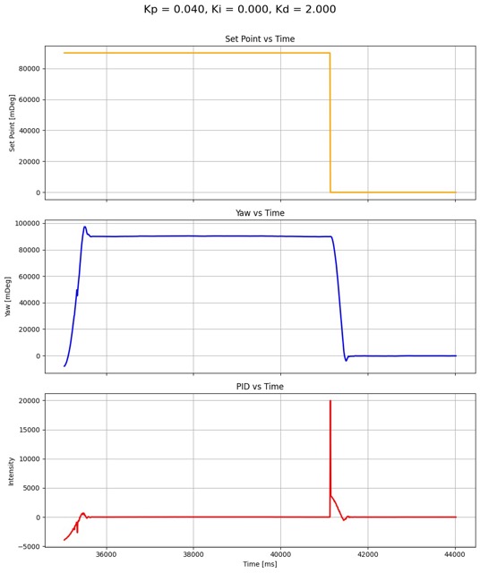
In the test data shown above, I changed the set point from 90 degrees to zero degrees at around 41500ms. The PID cranks up to an absurdly high value, caused by derivative kick, and rapidly moves the robot into the correct position. With such a large PWM spike, I would have expected a larger overshoot. However, the graph shows minimal overshoot and little to no oscillation at equilibrium. I have included two videos showing the successful implementation of orientation control. The first video shows me kicked the robot, attempting to perturb the robot from its set point. The video shows that the robot resists my kicks and aggressively recovers its set point.
The second video shows the set point of the robot being changed over time. The orientation is changed three times.
References
- Received help from Sophia Lin with changing the degrees per second parameter