Lab 5: Linear PID Control

Prelab

Bluetooth and Debugging Setup

Using the code from lab 3 as a starting point, I created new commands for PID control. First, I created a START_PID command. This command modifies global PID variables used in the controller. Eventually, I will implement the PID controller inside of this command.

case START_PID:
    success = robot_cmd.get_next_value(kp);
    if(!success){return;}
    success = robot_cmd.get_next_value(ki);
    if(!success){return;}
    success = robot_cmd.get_next_value(kd);
    if(!success){return;}
    break;

This allows me to tune the PID variables without reuploading the code every time. Then, I created a command that sends the PID data saved the the global arrays. This function is called SEND_PID_DATA.

case SEND_PID_DATA:
    Serial.println("Sending PID Data");
    for(int j = 1; j < MAX_SAMPLES; j++){
        tx_estring_value.clear();
        tx_estring_value.append(timeData[j]);
        tx_estring_value.append(" ");
        tx_estring_value.append(distanceData[j]);
        tx_estring_value.append(" ");
        tx_estring_value.append((int)PIDData[j]);
        tx_estring_value.append(" ");
        tx_estring_value.append(errData[j]);
        tx_characteristic_string.writeValue(tx_estring_value.c_str());
        tx_estring_value.clear();
    }
    Serial.println("Done Sending PID Data!");
    break;

Now that the Artemis can send time, distance, PID, and error data, I need to make sure my computer is set up to receive the data. Each type of data point in the transmission is separated by space, so I built a notification handler to parse the difference types of data into python arrays.

def notif_handler(uuid, byte_array):
    msg = ble.bytearray_to_string(byte_array)
    data = msg.split(" ");
    for i in range(4):
        if(i == 0):
            time_arr.append(int(data[i]))
        elif(i == 1):
            dist_arr.append(float(data[i]))
        elif(i == 2):
            pid_arr.append(float(data[i]))
        elif(i == 3):
            err_arr.append(float(data[i]))
    print("Data Received")
ble.start_notify(ble.uuid["RX_STRING"], notif_handler)

Finally, I created a python script to graph the data using Pyplot.

import matplotlib.pyplot as plt
fig, axs = plt.subplots(3, 1, figsize=(10, 12), sharex=True)
fig.subplots_adjust(hspace=0.3)  # Add some space between subplots

# Plot 1: Distance
axs[0].plot(np.arange(0,2000), dist_arr, color='blue', linewidth=2)
axs[0].set_title('ToF Distance vs Time')
axs[0].set_ylabel('Distance [mm]')
axs[0].grid(True)

# Plot 2: Error
axs[1].plot(time_arr, err_arr, color='red', linewidth=2)
axs[1].set_title('Error vs Time')
axs[1].set_ylabel('Error [mm]')
axs[1].grid(True)

# Plot 2: Error
axs[2].plot(time_arr, pid_arr, color='orange', linewidth=2)
axs[2].set_title('PID vs Time')
axs[2].set_ylabel('PID')
axs[2].set_xlabel('Time [ms]')
axs[2].grid(True)

fig.suptitle('Kp = 0.000, Ki = 0.000, Kd = 0.000', fontsize=16)
plt.tight_layout(rect=[0, 0, 1, 0.97])
plt.show()

Lab Tasks

The purpose of this lab was to achieve positional control using PID control. The goal is to have the robot drive as fast as it can towards a wall and stop when it is 1 foot away from it. I wanted the controller to support a wide range of starting distances, so I set the TOF sensor to long distance mode using distanceSensor1.setDistanceModeLong(). This also comes with the benefit of faster sensing.

Range/Sampling Time

By printing out the time after every PID calculation, I found that the ranging time is 100ms. I experimented using the Polulu library to shorten the ranging time, but anything under 100ms decreased the accuracy of the reading significantly. I could have low-passed the faster readings, but that would result in a delay in the PID controller. I also played around with setProximityIntegrationTime(), but found that the default settings were optimal for my system. I decided to keep the ranging time at 100ms for simplicity and reliability.

The PID loop runs significantly faster than the sensors acquire data. By printing the time in the main loop, I found that the loop runs at 2ms (500Hz). In later parts of the lab, we can use these extra cycles (where the sensor is not producing an output) to predict the robot’s position from the wall and continue to run PID calculations.

Deadband and Movement Functions

Since there is friction between the motor and the wheels, the robot can not move if PWM signal isn’t strong enough to drive the motors to overcome static friction. I foresee this becoming an issue when the PID system is near the equilibrium point, and the PWM signals become small. To find the minimum PWM signal needed to overcome static friction, I created two movement functions driveForward, driveBackward and stopMotor.

void driveBackward(int pwm){
  analogWrite(PIN1, pwm);
  analogWrite(PIN2, 0);
  analogWrite(PIN3, 0);
  analogWrite(PIN4, pwm);
}

void driveForward(int pwm){
  analogWrite(PIN1, 0);
  analogWrite(PIN2, pwm);
  analogWrite(PIN3, pwm);
  analogWrite(PIN4, 0);
}

void stopMotors(){
  analogWrite(PIN1, 0);
  analogWrite(PIN2, 0);
  analogWrite(PIN3, 0);
  analogWrite(PIN4, 0);
}

The combination of these three functions made it easy to test for the DEADBAND value, which is equal to the pwm variable just below where the motors start moving the robot forward. When the battery is fully charged, the value of DEADBAND is 30. I also used the stopMotor function as a hard stop in case the robot went out-of-control.

PID Controller

Shown below is the core logic of my PID controller. The code for acquiring distance and time data (current time and dt) is the same as lab 3. This code implements a basic PID controller, where Kp, Ki, and Kd are sent to the command via Bluetooth.

// calculate error derivitive
dError = (lastError - prevError) / dt;
prevError = lastError;

// calculate integral
integral = integral + lastError * dt;
integral = constrain(integral, -1000, 1000);
    
// put it all together
PIDData[i] = kp * lastError + ki * integral + kd * dError;

Now that I had calculated the PWN value, I needed to change the PWM signals set to the motors. I ended up reusing the deadband testing functions because the robot is only expected to move forward and backwards for this lab.

// apply motor control
if(PIDData[i] >= 5){
    driveForward((int)PIDData[i] + DEADBAND);
} else if(PIDData[i] <= -5) {
    driveBackward((int)abs(PIDData[i]) + DEADBAND);
}else{
    stopMotors();
}
i++;

Notice the DEADBAND offset is the same regardless of which direction the robot is driving.

Tuning Approach

To tune my PID system, I followed these steps:

1. Set Kp, Ki, and Kd to zero
2. Calculate theoritical value of Kp
3. Decrease Kp from calculated value until oscillation amplitudes are constant, and overshoot is minimized
4. Increase Ki until steady-state error is eliminated
5. Increase Kd to minimize oscillation amplitude

Proportional Controller Gain (Kp)

To set a proportional controller gain, I needed to consider, the range of motor values, the TOF sensor output range, and the desired system response. For PWM, the motor input is limited from 0 to 255. My Kp value needs to be scaled properly so that the maximum expected error times Kp doesn’t exceed this range.

\[\text{PWM} = \text{Kp} \times \text{error}\] \[\begin{align*} \text{max error} &= \text{maximum range} - \text{target distance}\\ &= \text{4000mm} - \text{304mm}\\ &= \text{3696mm} \end{align*}\] \[\text{Kp} = \frac{\text{PWM}}{\text{error}} = \frac{\text{255}}{\text{3696mm}} = 0.069\]

This does not mean that the system is optimally tuned at Kp = 0.069. It simply means that for the long setting on the distance sensor, Kp can not EXCEED 0.069. I ran a test for Kp = 0.069. The robot starts at around 1200mm from the wall and rapidly approaches the target position. There’s significant overshoot, where it almost hits the wall before it recovers, oscillates, and stabilizes around 304mm. The overshoot and oscillations show that Kp is too high.

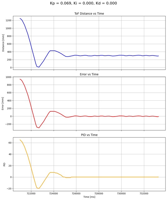
This video shows why overshooting the equilibrium point by too much is dangerous. If the robot slams into the wall too hard, it can mess up the orientation of the robot, making getting reliable sensor readings much harder.

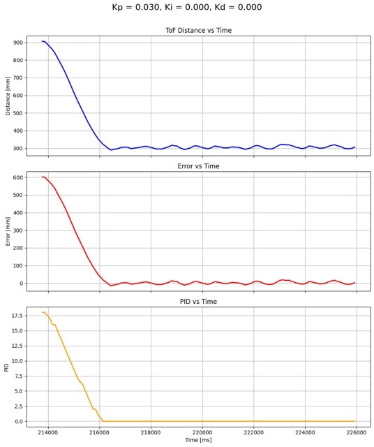
For the next couple of tests, I incrementally decreased Kp until I got a result that I was happy with. For each smaller value of Kp, the robot approached the wall slower, reducing overshoot. It also reduced the overall magnitude of oscillations. I was happy with the test for Kp = 0.069. The approach to the target is slower and smoother, there’s hardly any overshoot, and the control output decreases much more smoothly around equilibrium.

In this video, the robot moves noticeably slower because of the smaller Kp.

Integral Controller Gain (Ki)

The next step in the tunning process was to increase Ki from zero to eliminate steady-state error. Luckily, there was little to no steady state error for Kp = 0.030. This is because of the deadband offset, which prevent the robot from getting stuck at lower PWM calculations. Basically, the robot is able quickly recover from error, so error-build-up is negligible. Therefore, I decided that there was no need to increase Ki from zero, which also means that there was no need for integrator windup protection.

Derivative Controller Gain (Kd)

For the previous setpoint (Kp = 0.030, Ki = 0.000, Kd = 0.000), There is a small amount of overshoot and oscillation at steady state. The derivative controller can reduce both of these behaviors by applying a braking effect when the robot approaches the system too fast. I started by testing small values of Kd, such as 0.03 - 0.09, but did not notice a difference in the system. Then, I increase Kd to 10, which reduced oscillations significantly. My final value for Kd was 11, which was a good balance between dampening and responsiveness. The value for Kd was found mostly using trial-and-error.

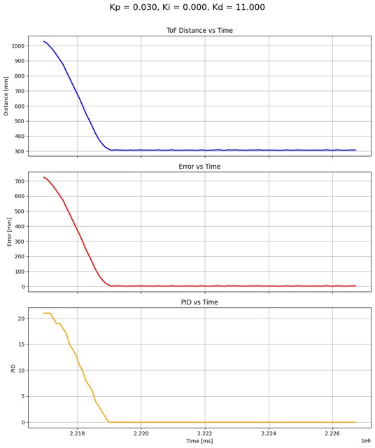
The distance graph shows the robot approaching the wall from around 1000mm, stabilizing around 304mm. The response shows a smooth approach without overshoot.The error graph shows that there is minimal steady-state error. The PID graph isn’t as clean as the distance and error graph, as it shows the controller’s effort to stabilize the non-ideal physical system. The robot’s braking behavior as it approaches the wall can be clearly seen in the video:

Extrapolation

The last part of this lab was to extrapolate new TOF values based on recent sensor values. This would allow the Artemis to run the PID loop faster, which enables the robot to the wall faster.

Step 1: Determine Loop Frequencies:

The ToF Sensor is returning new data at a rate of 1 measurement per 100ms, or 10Hz. I want to decouple the PID calculation loop from the sensor loop.

Step 2: Decouple Sensor Rate and PID Loop Rate To decouple the sensor rate and PID loop rate, I simply moved the PID calculations into an else-statement following the if-statement that checks if the data is ready. This means that distance variable is updated periodically (10Hz) but the PID calculations happen at a much faster rate in the else-statement. With this change, the behavior of the PID controller did not change.

prevTime = sensorTime;
prevErr = sensorDistance - 304;
distanceSensor1.clearInterrupt();
distanceSensor1.stopRanging();
distanceSensor1.startRanging();

while(i < MAX_SAMPLES){
// when data is ready
if(distanceSensor1.checkForDataReady()){
    // read distance
    distance = distanceSensor1.getDistance();
    prevSensorDistance = sensorDistance;
    sensorDistance = distance;
    prevSensorTime = sensorTime;
    sensorTime = millis();
    
    // restart sensor
    distanceSensor1.clearInterrupt();
    distanceSensor1.stopRanging();
    distanceSensor1.startRanging();
else{
    // run the PID loop anyways
}

Step 3: Loop Speed Compared to Sensor Rate

The PID control loop is now able to complete in 10ms, which corresponds to a frequency of 100Hz. Comparing this frequency to the sensor frequency of 10Hz, we find that the PID calculation loop runs tens times faster than the sensor loop.

Step 4: Estimate Distance Values

To predict distance data between sensor reads, I implemented a simple extrapolation algorithm.

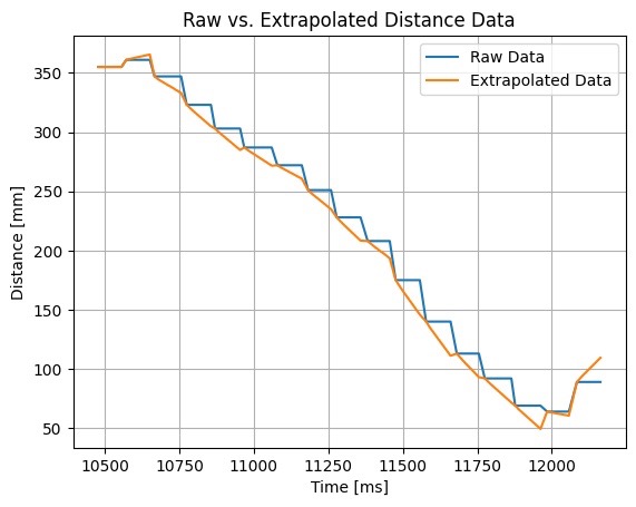
\[y = y_1 + (x-x_1)\frac{(y_2-y_1)}{(x_2-x_1)}\]

To implement this equation, I calculated the slope between two previous sensor calculations, multiplied it with the time since the last measurement, and added the product to the previous distance value.

extrapSlope = (sensorDistance - prevSensorDistance) / (sensorTime - prevSensorTime);
distance = sensorDistance + (millis() - sensorTime) * extrapSlope;

Shown below is a plot with corresponding raw and extrapolated data on the same graph. It shows that the raw data is moving in steps, with the extrapolated data is smoothly transitioning from one reading to the next.

This made a huge difference in the system. I was able to increase the maximum speed of my robot to 1 meter per second, and after re-tuning the system, ended with Kp = 0.08, Ki = 0.00, and Kd = 30.0.

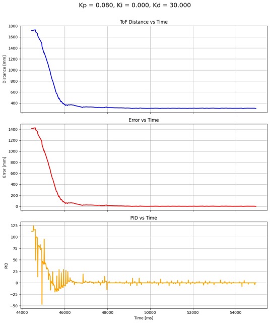
At faster speeds, the wheels of the robot skid, which means the distance data and PID data a lot more chaotic. Nonetheless, it approaches the wall with little to no overshoot at a much faster rate than before.

Three Repeated Experiments

Here are three successful runs of the PID system back-to-back to show reliability. Apologies for the piano music in the background. I was very tired and forgot to turn it off before recording.

References

• Consulted Ben Liao for decoupling the PID and sensor rates.
• Consulted Jeffery Cai for general coding advice
• Used Mikayla Lahr Course Webpage for getting a better idea of what graphs were needed