Lab 3: Time of Flight Sensors

Prelab

According to the datasheet, the I2C connection goes up to 400 kHz with fast mode. The I2C address is 0x52 by default, but can be set programmatically.

Using Multiple ToF Sensors

Since the two ToF sensors share the same I2C address by default, they can not send data in parallel through that same address. One option would be to continuously enable/disable the two sensors, letting them send data in turns. Although simple to implement, this method has the downside of low sampling rate. Instead of that, I will change the two sensors’ addresses programmatically. This is done by using the XSHUT pin to shut down one of the ToF sensors, changing its address, and then powering it on. This allows the two ToF sensors to send data through different I2C channels in parallel.

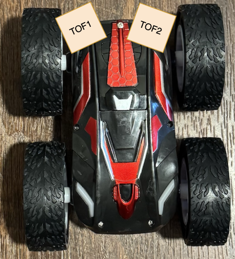
ToF Sensor Placement

The two ToF sensor should be placed at the front of the robot, one closer to the left and the other closer to the right. Usually, the front sensors should be angled upwards (not too much relevant information on the floor), but since the robot is able to flip, postioning them directly foward offers more consistent detection overall. This postioning allows the two sensors to work together for reliable forward obstacle detection. Detection during turns would be achieved by individual sensors, depending on the direciton of the turn.

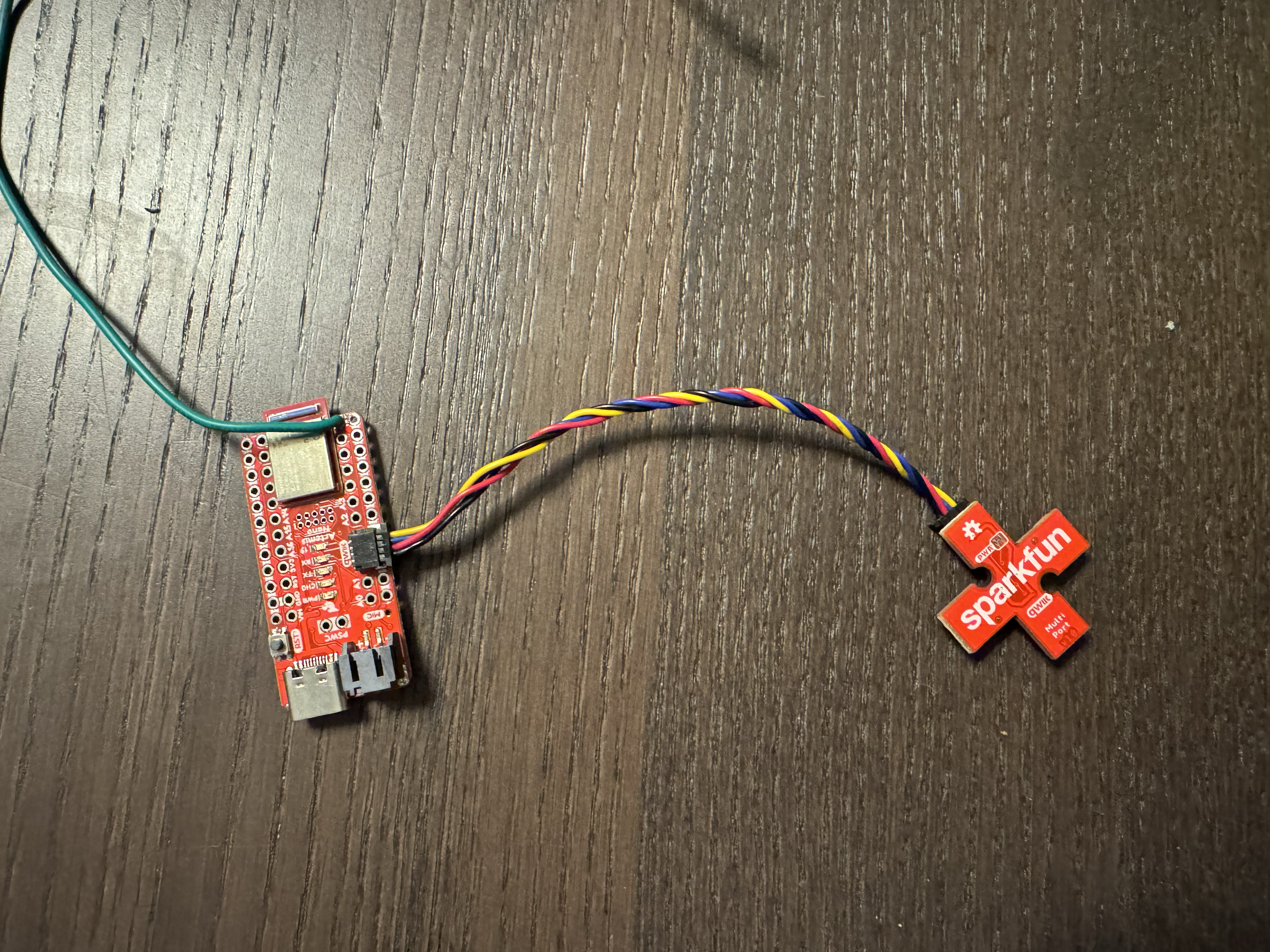
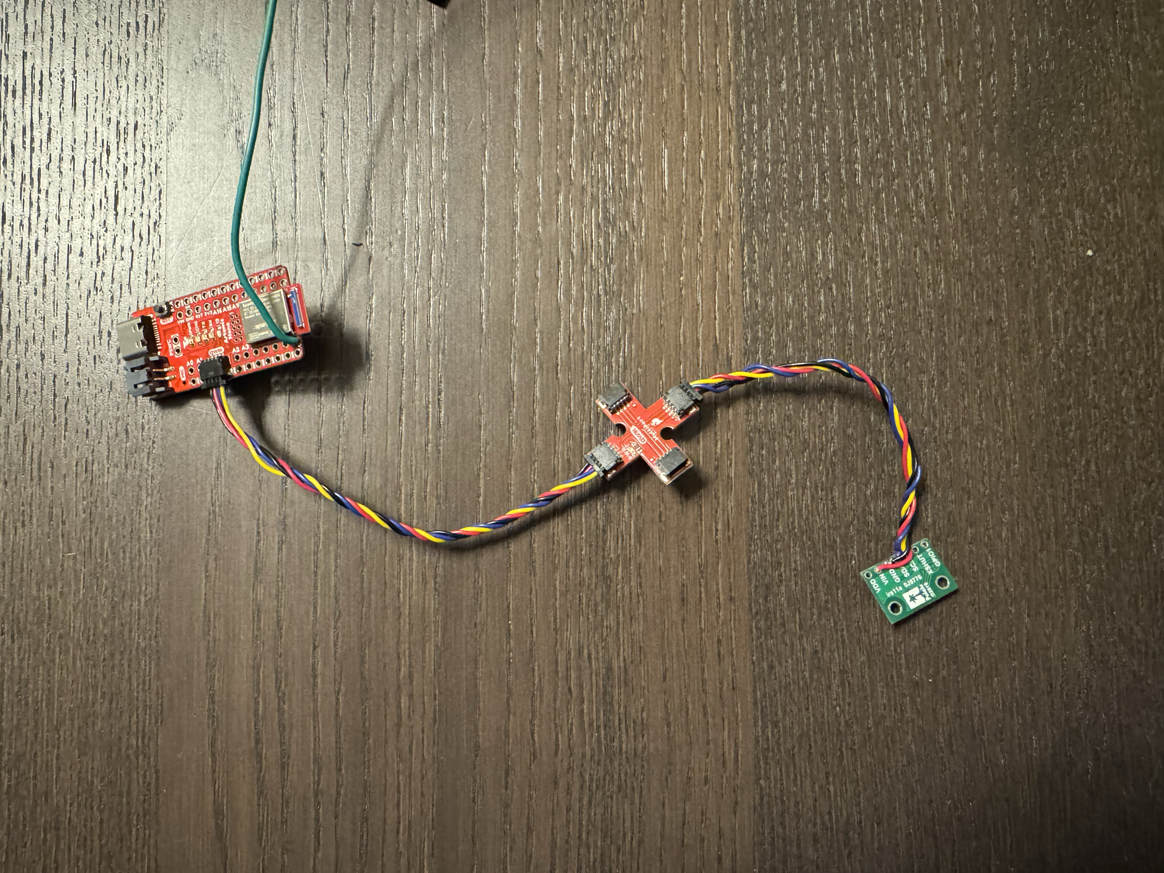
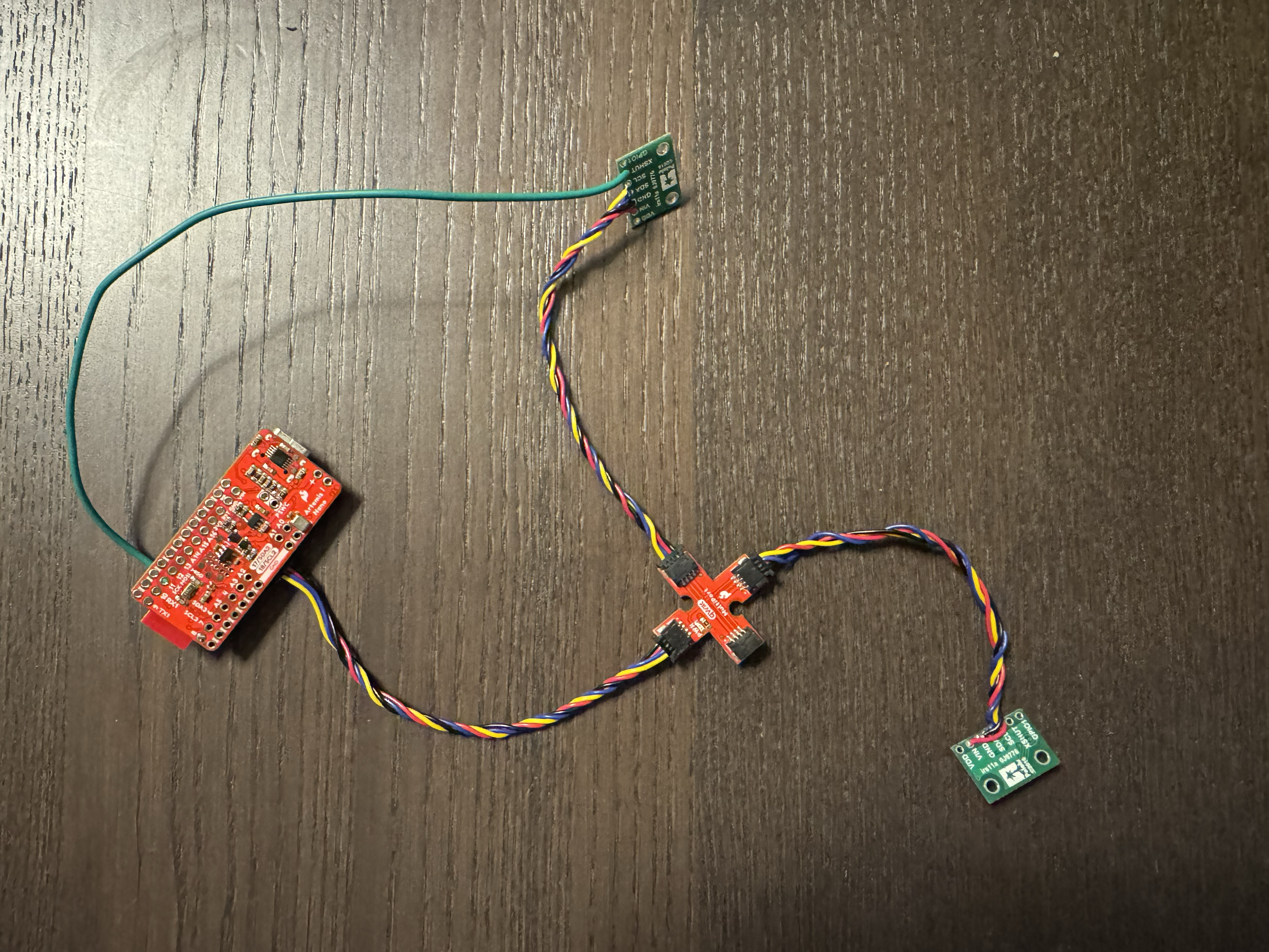
Wiring Diagram

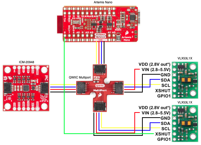
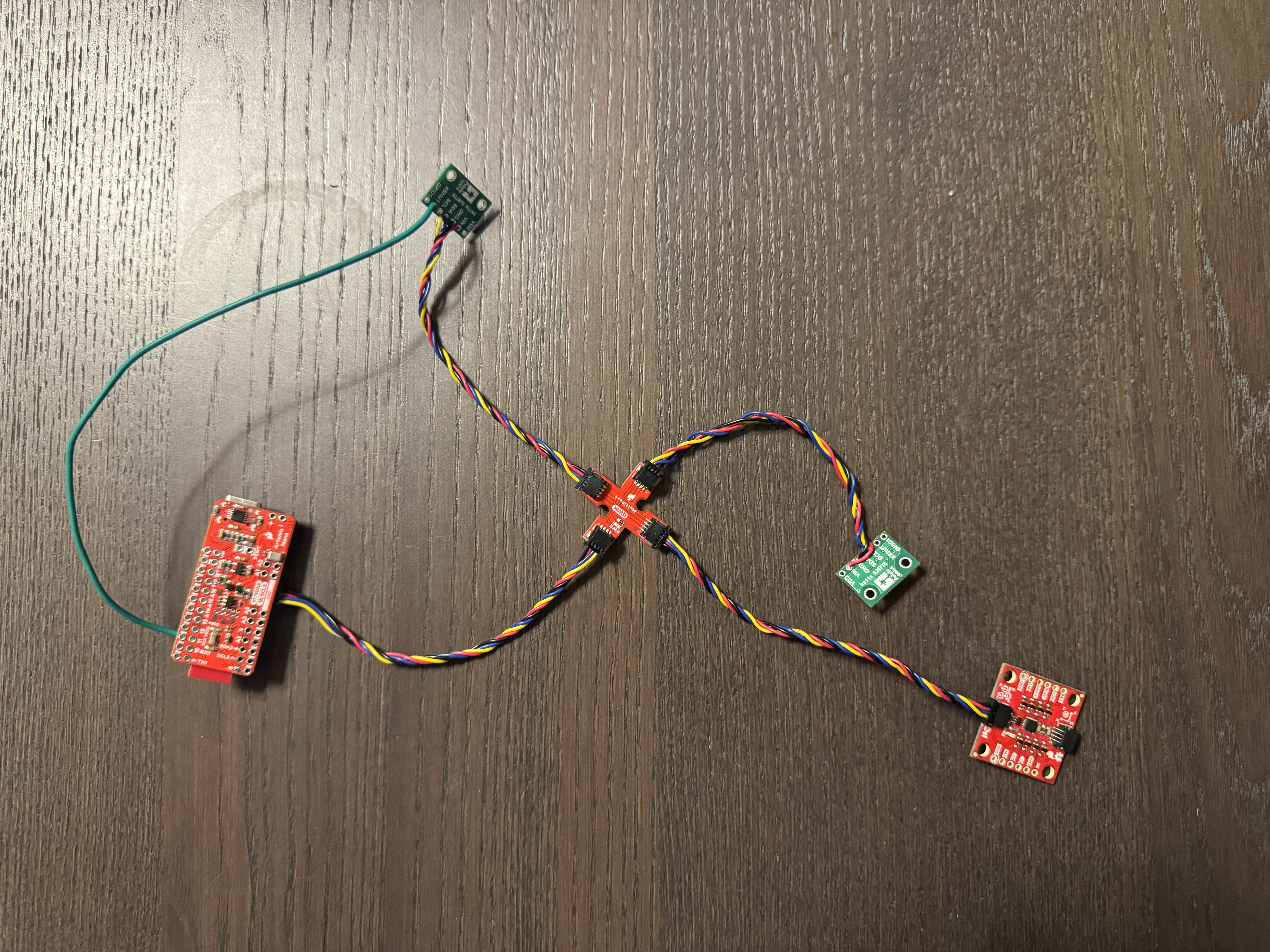
The diagram below shows how the ToFs and IMU should be wired to the Artemis Nano. The QWIIC breakout board increases the number of QWIIC connections from 1 to 3, which is need for the 2 ToF sensors and the IMU. The XSHUT jumper wire is only connected to one of the ToFs because only one has to be assigned a unique address.

Lab Tasks

Task 1: Power Artemis with Battery

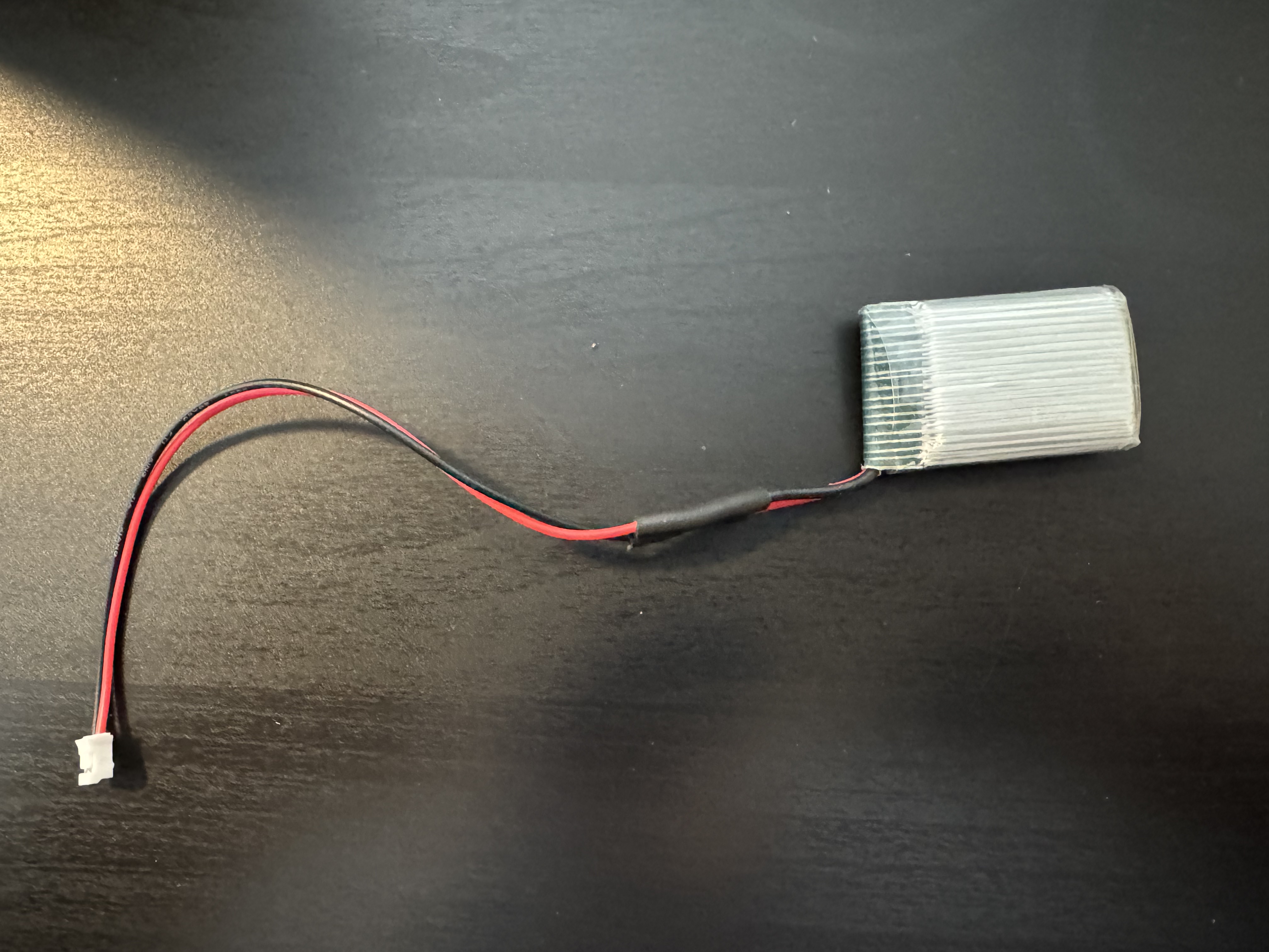
Before I could power the Artemis Nano with the battery, I needed to change the connector on the battery. To do this, I cut off the previous connector and soldered on a new connector. I had to solder together different colored wires because the wire color on the connector does not mean anything. I made sure to secure the soldering job using shrink wrap, as shown below.

The video below demonstrates the Artemis being powered by a battery and its ability to still receive and send messages.

Task 2: Install Arduino Library

This is the specific Arduino library that must be installed for the ToF sensors to work properly.

Task 3: QWIIC Break-out Board to Artemis

I connected the QWIIC breakout board to the Artemis. This expands the number of QWIIC ports from one to three. No soldering was required for this.

Task 4: Single ToF to QWIIC Break-out Board

Then, I connected a ToF sensor to the QWIIC breakout board. Since the ToF sensor doesn’t have a QWIIC connection port, soldering is needed. I trimmed the plug off of a QWIIC connector and soldered the wires directly to the sensor. The wires are VIN (red), GND (black), SDA (blue), and SCL (yellow).

Task 5: Scan the I2C channel

To find the address of the sensor, I used the example code for I2C. Upon running the code, the Artemis started scanning for I2C devices and found the one ToF sensor at address 0x29.

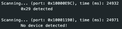
Since I2C uses the least significant bit of the address to indicate read/write, the actual address is found by bit-shifting to the left by one bit.

0x29 in binary is 00101001. After the bit-shift, the result is 01010010, which is 0x52 (what we expect from the datasheet).

Task 6: ToF Mode

Shown below are several tables from the ToF sensor datasheet that outline the reliable range under different lighting conditions.

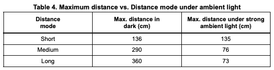
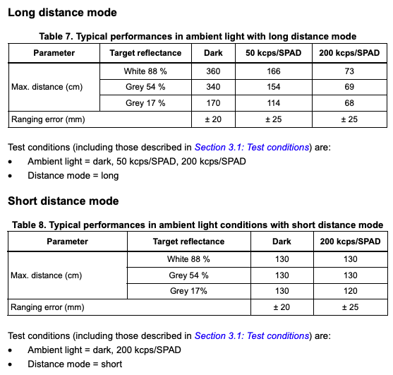
From table 4, we can see that the short distance mode has similar maximum range in darkness and strong ambient light. Meanwhile, medium and long distance mode has substantially less range under strong ambient light compared to darkness.

From table 7 and table 8, we can see that typical performance in long distance mode is highly variable based on different conditions, while short distance mode maintains a consistent performance range of 130 cm.

Short Mode:

• Pros: performance is consistent across lighting conditions, more granular data
• Cons: generally shorter range

Medium Mode:

• UNAVAILABLE

Long Mode:

• Pros: generally longer range
• Cons: performance is inconsistent across lighting conditions

Given the pros and cons, I think short mode is better for the final robot. A longer range means nothing if the performance is inconsistent. Also, short distance mode has higher data granularity within its effective range than long distance mode.

Task 7: Test Chosen Mode

There are several steps to sample data from the ToF sensor. First, I used the startRange() method to tell the sensor to start measuring the distance. This data takes some time to acquire, so the program stays in the loop for as long as the result is not available. When I confirm that the data is ready using checkForDataReady, I append the data to the appropriate arrays and restart the process, until MAX_SAMPLES number of data points have been aquired.

while(i < MAX_SAMPLES){
  distanceSensor1.startRanging(); 
  if(distanceSensor1.checkForDataReady()){
    int distance = distanceSensor1.getDistance(); the sensor
    distanceSensor1.clearInterrupt();
    distanceSensor1.stopRanging();
    timeData[i] = (int)millis();
    tof1Data[i] = distance;
    i++;
  } 
}
Serial.println("Done Reading Single TOF Data.");
Serial.println("Sending Single TOF Data...");
Serial.print("[");
for(int i = 0; i < MAX_SAMPLES; i++){
    Serial.print(tof1Data[i]);
    Serial.print(",");
}
Serial.print("]");
Serial.println("Finished Sending Single TOF Data!");
break;

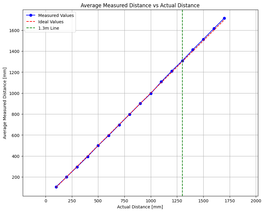
Using this code, I set MAX_SAMPLES to 10, and took measurements using my wall as an endpoint. I would take 10 measurement every 10cm, which was enough to get a good idea of the range, accuracy, repeatability, and ranging time. Here is the python list that I stored the data in.

data = [[104,106,103,106,106,106,106,103,104,105]
        ,[201,199,199,202,202,200,202,198,199,200]
        ,[296,297,298,296,296,296,295,297,297,297]
        ,[395,394,394,391,394,395,395,394,397,394]
        ,[499,501,500,499,499,499,499,499,500,500]
        ,[596,596,595,594,594,597,596,596,597,594]
        ,[696,698,699,698,696,696,696,699,700,698]
        ,[797,798,799,798,799,800,799,799,797,797]
        ,[899,898,897,901,902,900,899,901,901,900]
        ,[995,997,995,996,997,994,995,994,995,995]
        ,[1109,1107,1107,1108,1108,1106,1106,1109,1108,1107]
        ,[1211,1209,1210,1211,1210,1214,1209,1214,1212,1212]
        ,[1308,1309,1308,1307,1309,1307,1308,1308,1310,1309]
        ,[1412,1411,1414,1415,1415,1417,1413,1413,1415,1413]
        ,[1513,1513,1514,1515,1512,1514,1515,1515,1512,1512]
        ,[1616,1615,1614,1615,1615,1615,1616,1614,1615,1618]
        ,[1716,1719,1712,1715,1713,1713,1715,1716,1716,1719]]

Range

The measurements are close to idea from 10mm to 1200mm. Starting at 1200mm, I started to see around 10mm of inaccuracy. As the distance increased past 1300mm, the measured distance deviated further and further away from idea. Playing on the conservative side, I would consider the range of distances from 0mm to 1300mm to be measured reliably.

Accuracy

The difference graph shows the sensor’s accuracy, and lack therof, as the actual distance increased. Since the robot itself is not that long, so a difference of 1 cm can be quite signifigant. However, higher error at a large distance away is acceptable if the robot has time to resample the data as the distance becomes shorter and more reliable.

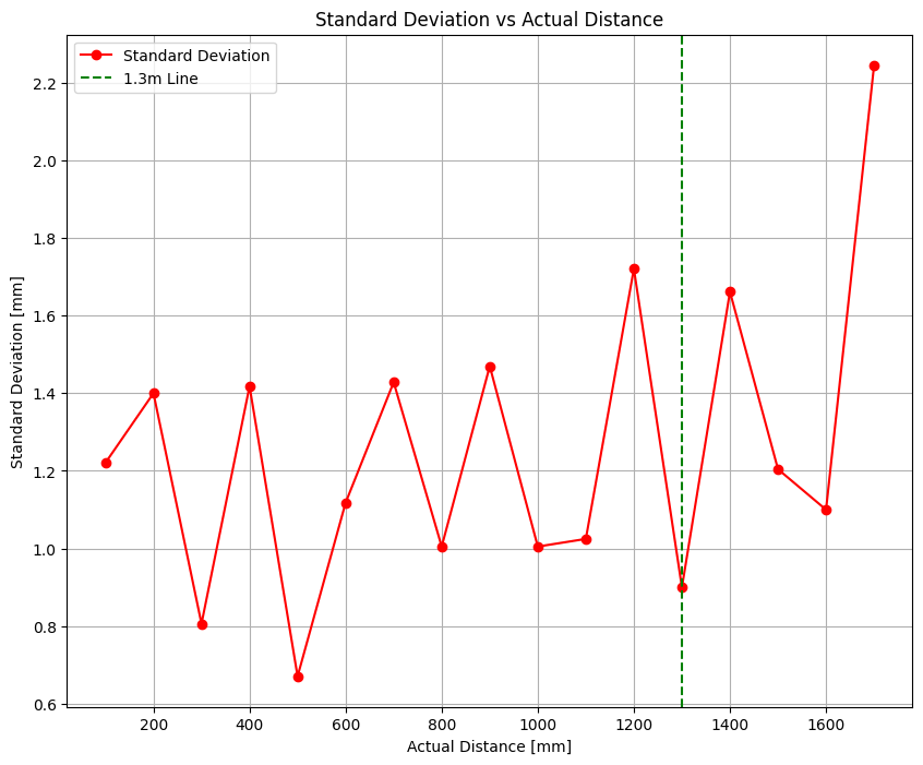
Repeatability

Shown below is the standard deviation vs actual distance graph. For my data, the standard deviation was fairly low, indicating that the sensor performs well in terms of consistency. At 1700mm, the standard devation spiked, which is to be expected because 1700mm is outside of the reliable range in short distance mode.

Ranging Time

In addition to printing out the distances, I added a loop to print the time in milliseconds. From the output, it can be seen that the ranging time is about 53 milliseconds, although this number was not always consistent for each measurement.

Distance 1: 57
16725
16732
16737
16744
16751
16759
16766
16770
Distance 1: 56
16778

Task 8: Two ToF Sensors Simultaneously

The XSHUT pin turns off the second ToF sensor when the pin is pulled LOW. To connect XSHUT on the MCU to the sensor, I soldered a jumper wire from the Artemis to the ToF sensor.

To set up the second sensor, I set the XSHUT pin to LOW shut down the second sensor. Then, I change its I2C address to an unused addressc. Finally, I set XSHUT back to HIGH, turning the sensor back on. This allows the two ToF sensors to send data through different I2C channels in parallel.

// shut down ToF Sensor 2
    digitalWrite(XSHUT, LOW);

    // initialize wire library
    Wire.begin();
    
    // start serial terminal 
    Serial.begin(115200);
    while(!Serial){
      ;
    }

    // set sensor 1 address
    distanceSensor1.setI2CAddress(ADDRESS);
    Serial.print("New Distance Sensor 1 Address: 0x");
    Serial.println(distanceSensor1.getI2CAddress(), HEX);
    if (distanceSensor1.begin() != 0){
      Serial.println("Sensor failed to begin.");
      while (1);
    }

    // turn on sensor 2, which is set to the default address
    digitalWrite(XSHUT, HIGH);
    Serial.print("New Distance Sensor 2 Address: 0x");
    Serial.println(distanceSensor2.getI2CAddress(), HEX);
    if (distanceSensor2.begin() != 0){
      Serial.println("Sensor failed to begin.");
      while (1);
    }

After setting up the two ToF sensors wiht unique address, sampling data from them was very similar to how it was done with only one sensor. I created a new array to hold the data for the second sensor.

while(j < MAX_SAMPLES){
  distanceSensor1.startRanging();
  distanceSensor2.startRanging(); 
  if(distanceSensor1.checkForDataReady() && distanceSensor2.checkForDataReady()){
    int distance1 = distanceSensor1.getDistance(); 
    int distance2 = distanceSensor2.getDistance(); 
    distanceSensor1.clearInterrupt();
    distanceSensor1.stopRanging();
    distanceSensor2.clearInterrupt();
    distanceSensor2.stopRanging();

    timeData[j] = (int)millis();
    tof1Data[j] = distance1;
    tof2Data[j] = distance2;

    Serial.print("Distance 1: ");
    Serial.println(distance1);
    Serial.print("Distance 2: ");
    Serial.println(distance2);
    j++;
  }
}

Task 9: Code Execution Speed

Like the lab manual instructs, this program doesn’t use delays and instead checks if the data is ready using checkForDataReady(). Otherwise, it just keeps looping and a sample is not written to the array.

distanceSensor1.startRanging();
  distanceSensor2.startRanging(); 
  if(distanceSensor1.checkForDataReady() && distanceSensor2.checkForDataReady()){
    int distance1 = distanceSensor1.getDistance(); 
    int distance2 = distanceSensor2.getDistance(); 

In addition to printing out the distances, I added a loop to print the time in milliseconds. From the output, it can be seen that the ranging time is about 53 milliseconds, although this number was not always consistent for each measurement.

Distance 1: 57
16725
16732
16737
16744
16751
16759
16766
16770
Distance 1: 56
16778

This output shows that the MCU is running much faster than the sensor is producing values, which is a good time. I did the same thing for the function that uses two ToF sensors, and the ranging time expected doubled, to 100ms. The current limiting factor is the ranging time of the sensor, which is hard to optimize without making hardware changes.

Task 10: Sending over Bluetooth

for(int j = 1; j < MAX_SAMPLES; j++){
  tx_estring_value.append(timeData[j]);
  tx_estring_value.append(" ");
  tx_estring_value.append(tof1Data[j]);
  tx_estring_value.append(" ");
  tx_estring_value.append(tof2Data[j]);
  tx_characteristic_string.writeValue(tx_estring_value.c_str());
  tx_estring_value.clear();
}

Sending the data over Bluetooth just involved modifiying the Lab 1 code to support new variables. The time is listed first, then the sensor1 data, and then the sensor 2 data. Each data point is seperated by a space so that the notification handler knows where one data point ends and another starts.

def notif_handler(uuid, byte_array):
    msg = ble.bytearray_to_string(byte_array)
    print(msg)
    data = msg.split(" ");
    for i in range(3):
        if(i == 0):
            time_arr.append(int(data[i]))
        elif(i == 1):
            tof1_arr.append(int(data[i]))
        else:
            tof2_arr.append(int(data[i]))
ble.start_notify(ble.uuid['RX_STRING'], notif_handler)

Task 11: ToF Data vs Time

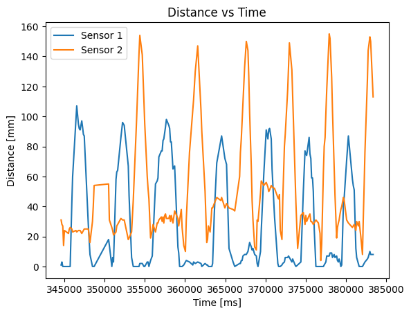
The results of the work from the previous section are shown below. The two sensors are able to send data in parallel. For this example, I only recorded around 4 seconds of data, but the program is able to do much more.

Task 12: IMU Data vs Time

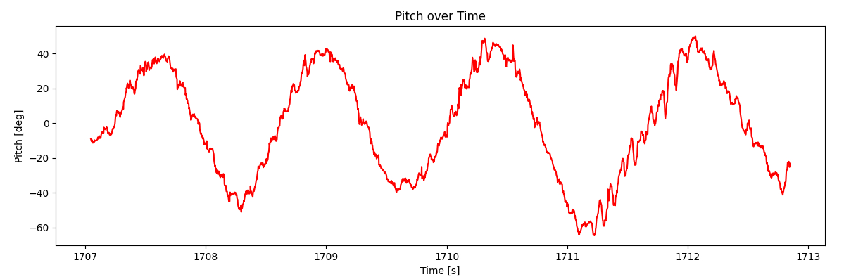
Finally, I used the last available port on the QWIIC breakout board to connect the IMU sensor to the Artemis, allowing for the collection of pitch, roll, and yaw data again. Shown below is a graph of unfiltered pitch angle over time. At this point, I can simulataneously acquire data from 2 ToFs and 1 IMU.

References

• Used Mikayla Lahr Course Webpage for general report layout inspiration
• Used Wenyi Fu Course Webpage for setting up the second ToF sensor