Lab 2: Inertial Measurement Unit

Setup the IMU

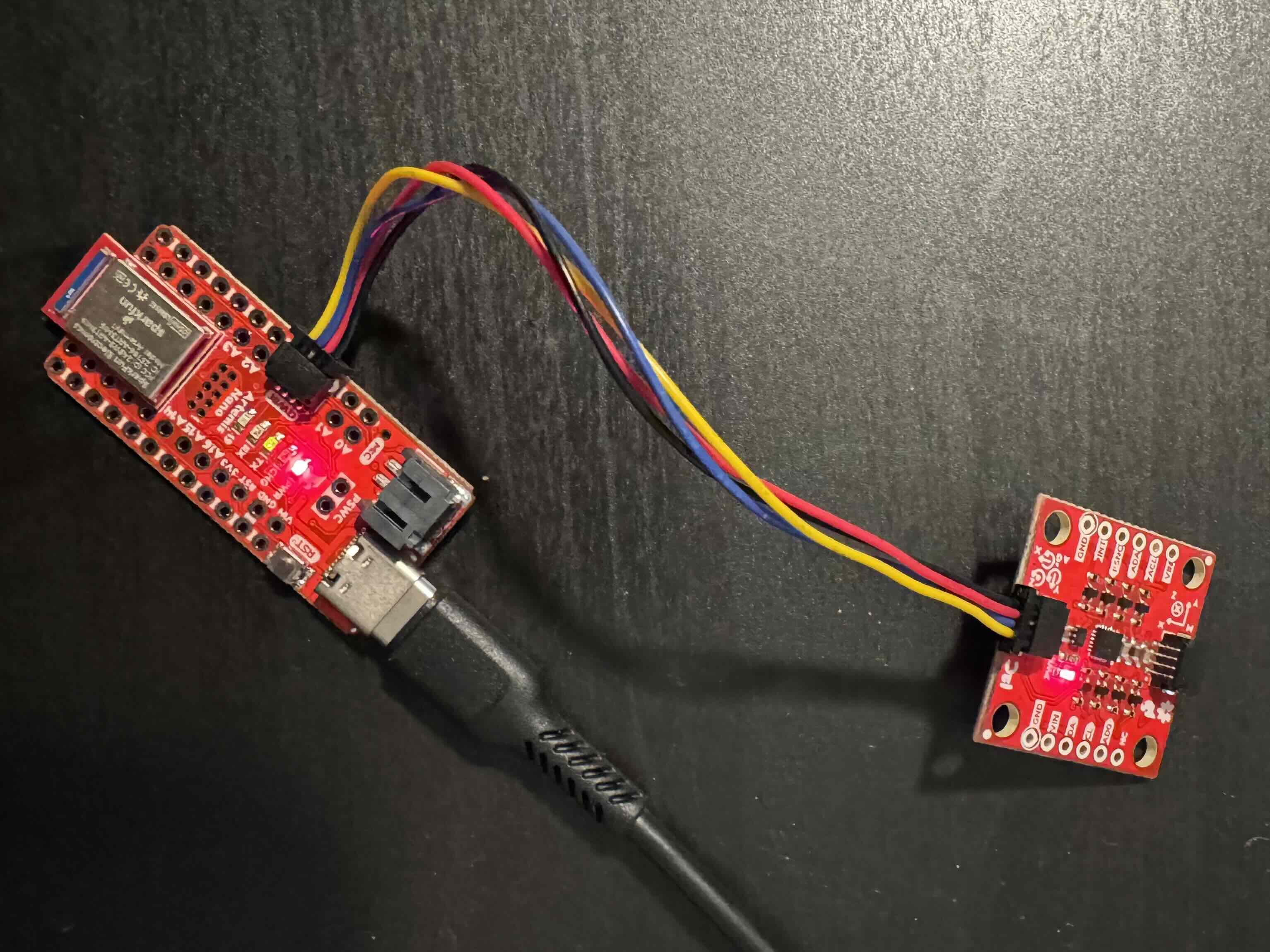
I connected the I2C connector on the IMU to the Artemis Nano using the braided QWIC connector.

Then, I installed the SparkFun ICM-20948 library in the Arduino IDE and ran the example code.

AD0_VAL defines the last bit of the IMU’s I2C address. Since we are only using one IMU in this lab, AD0_VAL should be set to the default of 1. Being able to change the I2C address on the IMU allows for the daisy-chaining of multiple IMUs stemming from the same I2C connection.

When the board is placed flat on the table, it experiences no acceleration in the x and y directions, but it is pulled downwards in the z-direction by gravity. In the beginning of the serial plot video above, we can see that the acceleration value in the z-direction is around 1000, while x and y are at 0. The x, y, and z values on the serial plotter are higher when the respective axis feels the pull of gravity, or some other force.

While the accelerometer measures linear acceleration, a gyroscope measures angular velocity. This means that an ideal gyroscope will produce all zero outputs if the board is stationary, but will produce an output at the appropriate axis if moved.

I added a visual indication that the board is running by blinking the LED three times on startup. I did this using the same BlinkWithoutDelay example code as lab 1.

if (currentMillis - previousMillis >= interval && blinks < BLINKS_ON_STARTUP) {
    // save the last time you blinked the LED
    previousMillis = currentMillis;

    // if the LED is off turn it on and vice-versa:
    if (ledState == LOW) {
        ledState = HIGH;
    } else {
        ledState = LOW;
        blinks = blinks + 1;
    }
    // set the LED with the ledState of the variable:
    digitalWrite(ledPin, ledState);
}

Accelerometer

I used the equations from class to convert accelerometer data into pitch and roll. Sadly, yaw can not be calculated from accelerometer data, but can be done using the gyroscope.

theta = atan2(myICM.accX(), myICM.accZ())  * (180.0 / M_PI); // Pitch
phi = atan2(myICM.accY(), myICM.accZ())  * (180.0 / M_PI);   // Roll

Pitch and Roll

When either pitch or roll are moved past its extremes (-180° or 180°), the reading will flip to the opposite extreme and move towards zero if the movement continues. This flipping behavior causes some instability in reading either pitch or roll when roll or pitch is set to 90°, respectively. This can be seen in the data below.

Pitch = 0, Roll = -90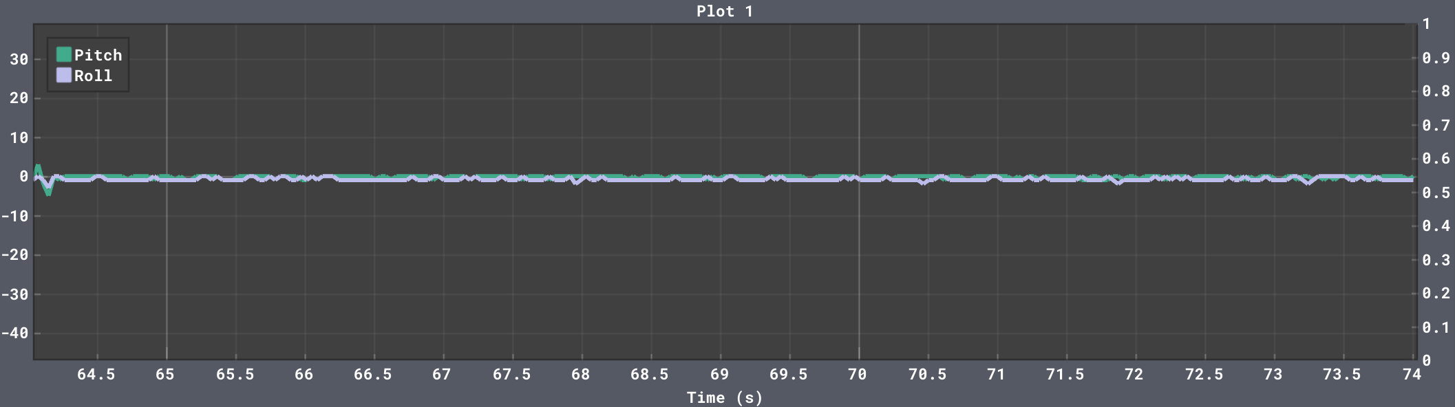

Pitch = 0, Roll = -90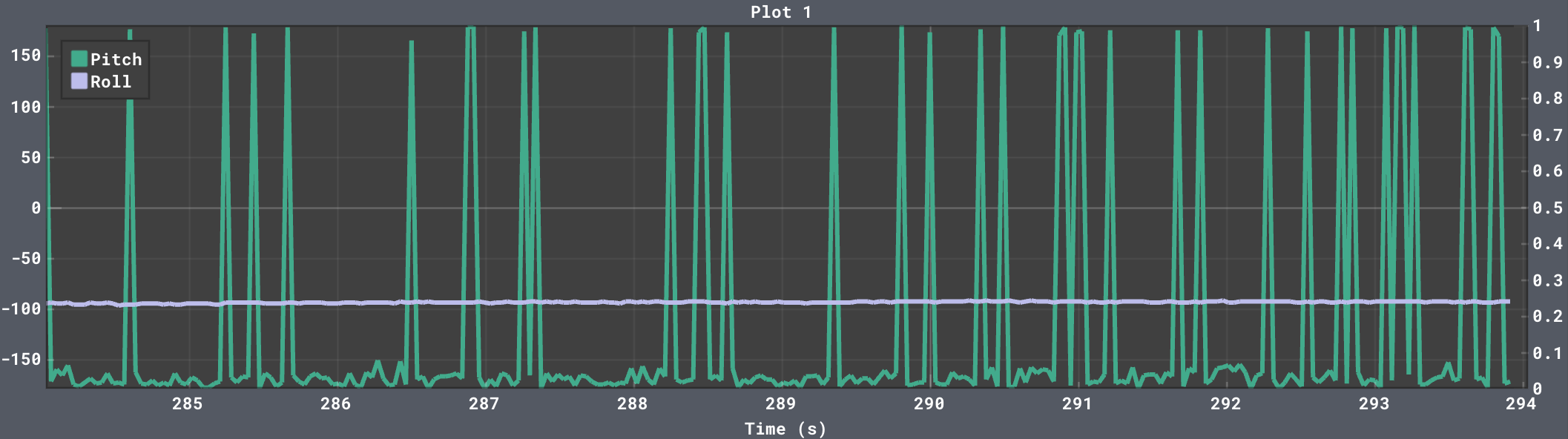

Pitch = 0, Roll = 90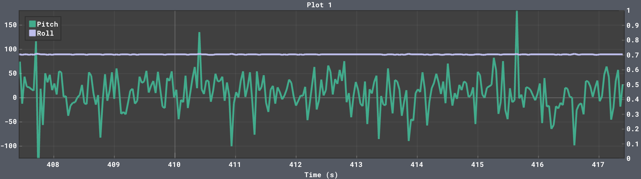

Pitch = 90, Roll = 0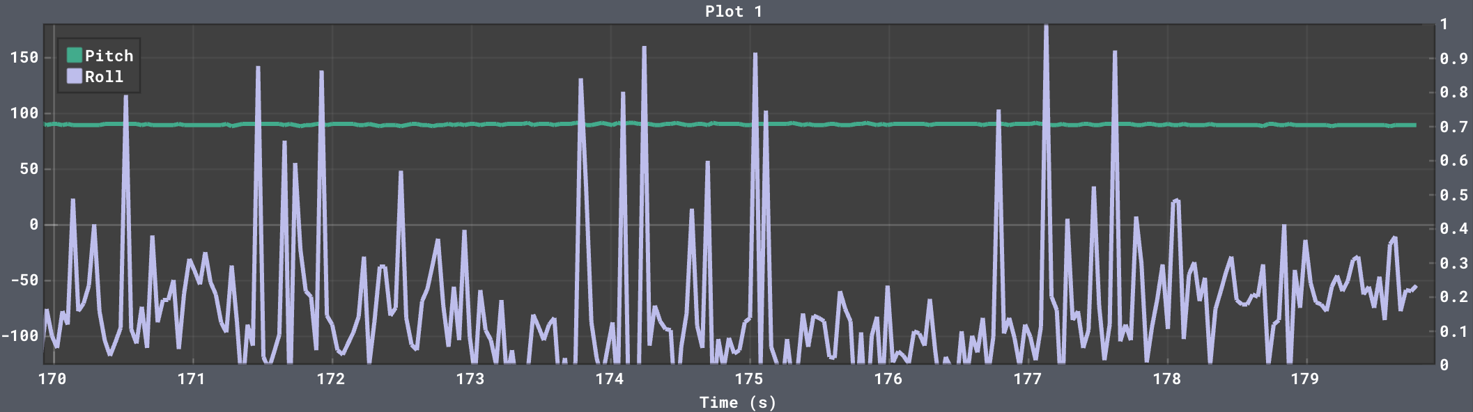

Pitch = -90, Roll = 0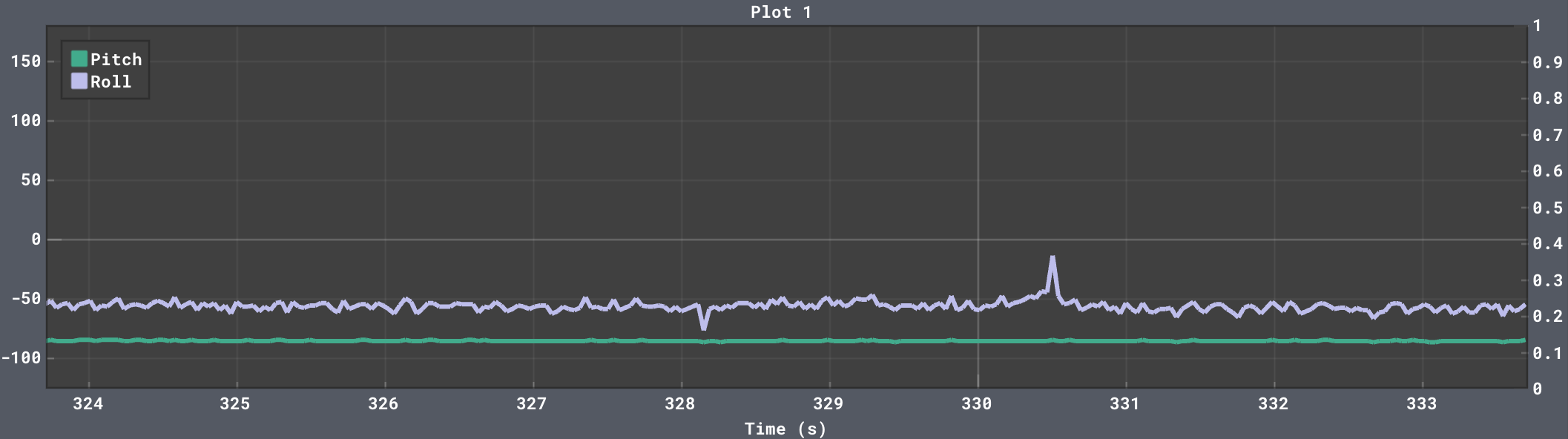

Strangely enough, the noisy flipping did not happen in this last case, which may have something to do with how the accelerometer is set up internally.

Jupyter Plotting

I used Bluetooth to send accelerometer data from the board to my PC. To capture 5 seconds of data, around 2000 data points are needed. It took around 58 seconds to send each point individually, which made testing tedious. To solve this problem, I appended several data points to each transmission and modified my notification handler to parse the data and organize it into arrays. Then, it was easy to plot the time domain graph using Matplotlib. Sending the data in batches of 3-5 decreased the transmission time to 10-15 seconds.

Accuracy

My accelerometer is accurate within 5 degrees of error. To perform a two-point calibration, I measured two known angles (-90 degrees and 90 degrees). Then, I assumed that the sensor is linear between these two points, and created a calibration equation to ensure accuracy. I do this for both pitch and roll. Here is the sample code for pitch calibration. Roll calibration is done the same way.

float calibratedPitch(float reading){
  float A1;
  float A2; 
  float m;
  float b;

  A2 = 86;
  A1 = -87;
  m  = 180.0 / (A2 - A1);
  b = - 90 - m * A1 ;

  return m * reading + b;
}

I did not use two-point calibration in the later sections of this lab because A1 and A2 should be set after it is attached to the robot.

Noise & FFT Analysis

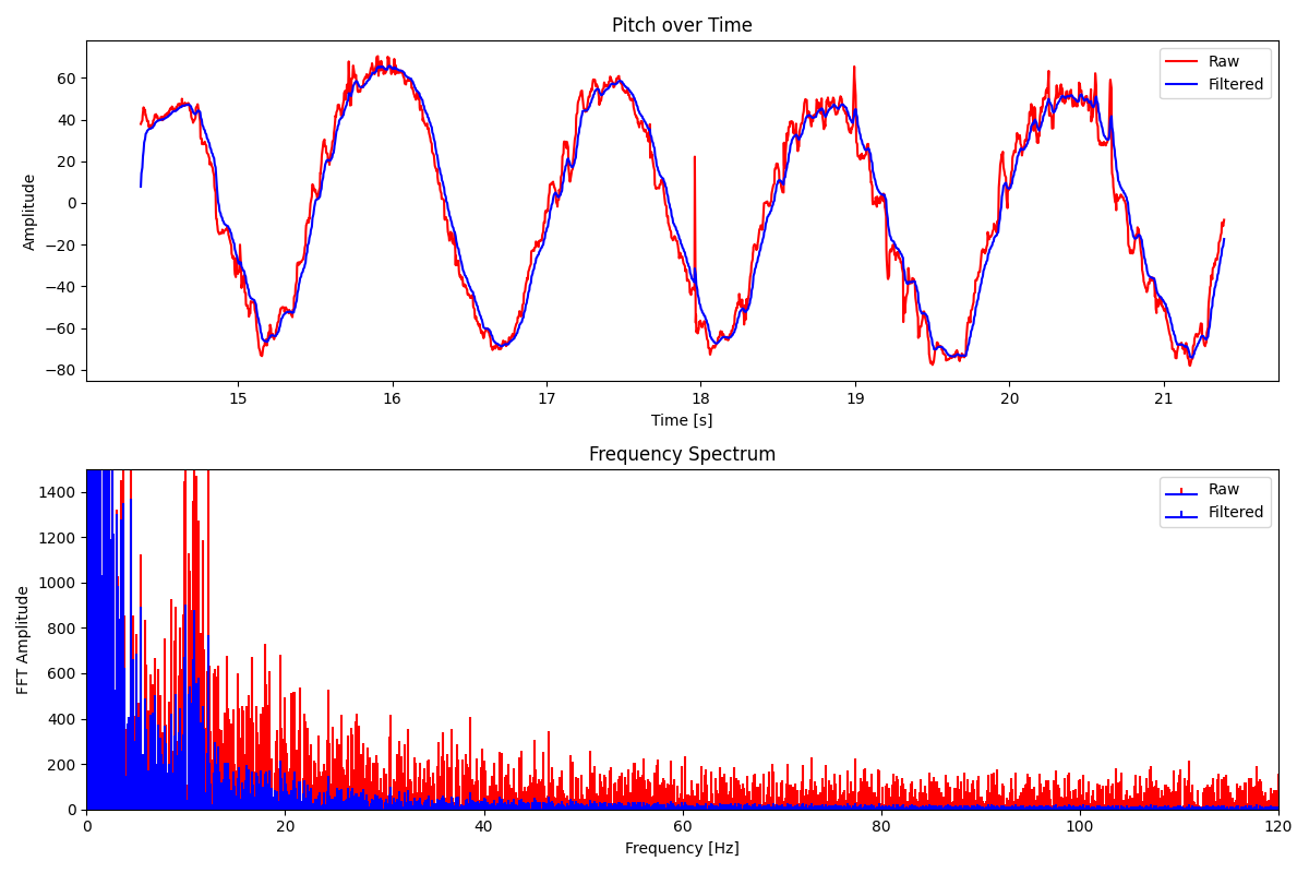
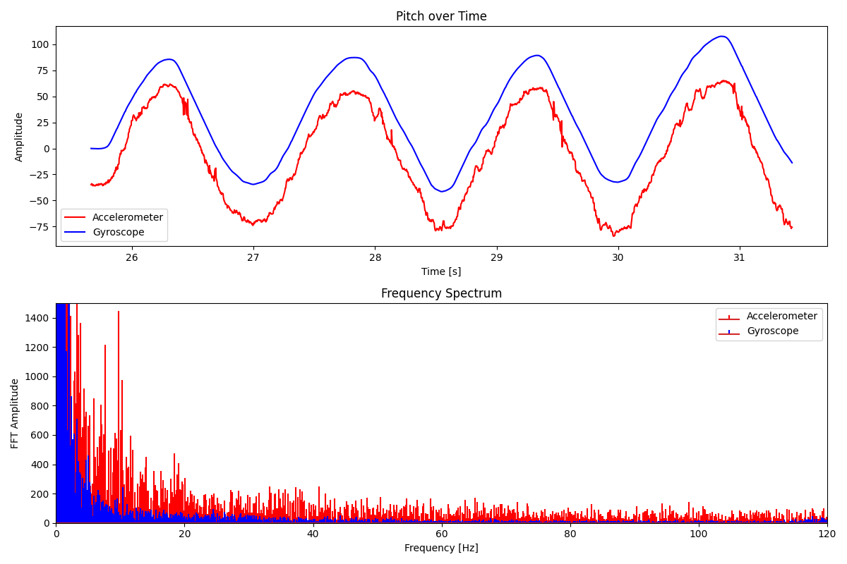
Shown below are the time domain and frequency domain graphs for the pitch while wobbling the IMU back and forth, with the RC car in its proximity.

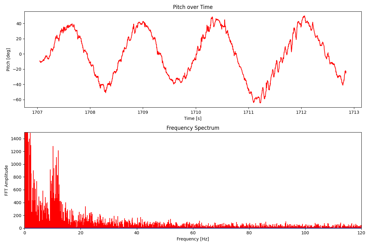
The time-domain signal tracks the movement pretty accurately, but the edges are jagged, revealing the sensor’s sensitivity to high-frequency motor noise. I think there is relatively low noise because there is already a hardware low-pass filter built-in. Looking at the frequency domain above, we can see two spikes. The spike at 1-2 Hz is the intended wobbling motion. The 10 Hz spike is the motor vibration. To get a better idea of where to set the cutoff frequency, I decided to induce some random vibrational noise by hitting the table at random intervals.

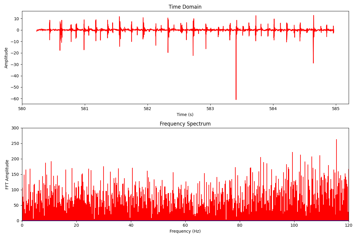
The spikes in roll are when I hit the table, and it’s seemingly random whether it spikes up or down. I decided to set the cut-off frequency to 10Hz. It would be sufficient to cut out the majority of high-frequency noise, while preserving intentional movements. Here is the calculation of alpha:

\[f=\frac{1}{2\pi RC}\] \[RC=\frac{1}{2\pi 10} = 0.0159154943092\] \[T=0.002\] \[\alpha=\frac{T}{T+RC}\] \[\alpha=\frac{0.002}{0.002+0.0159154943092}=0.11\]

Simple Lowpass Filter

Using this value of alpha, I implemented my low-pass filter to achieve the results shown below:

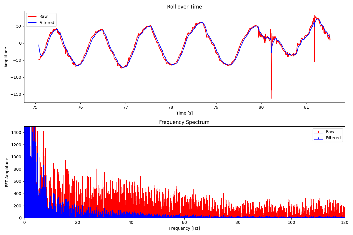
The low pass filter was able to significantly reduce noise in pitch and roll. The 10 Hz motor noise is much less problematic with the low pass filter.

Gyroscope

I found the roll, pitch, and yaw from the equations from class.

dt = (micros() - last_time)/1000000.;
last_time = micros();

pitch_g = pitch_g + myICM.gyrY()*dt;
roll_g = roll_g + myICM.gyrX()*dt;
yaw_g = yaw_g + myICM.gyrZ()*dt;

To test my implementation, I rotated the IMU along the pitch, roll, and yaw axises, in that order, as shown below.

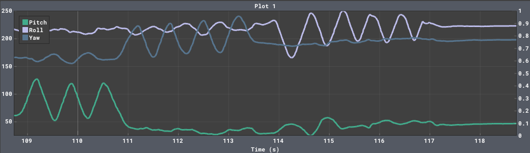
The drifting is severe in this screenshot, but the incremental changes are accurate and low-noise, which is all we need for the complementary filter.

Comparision to Accelerometer

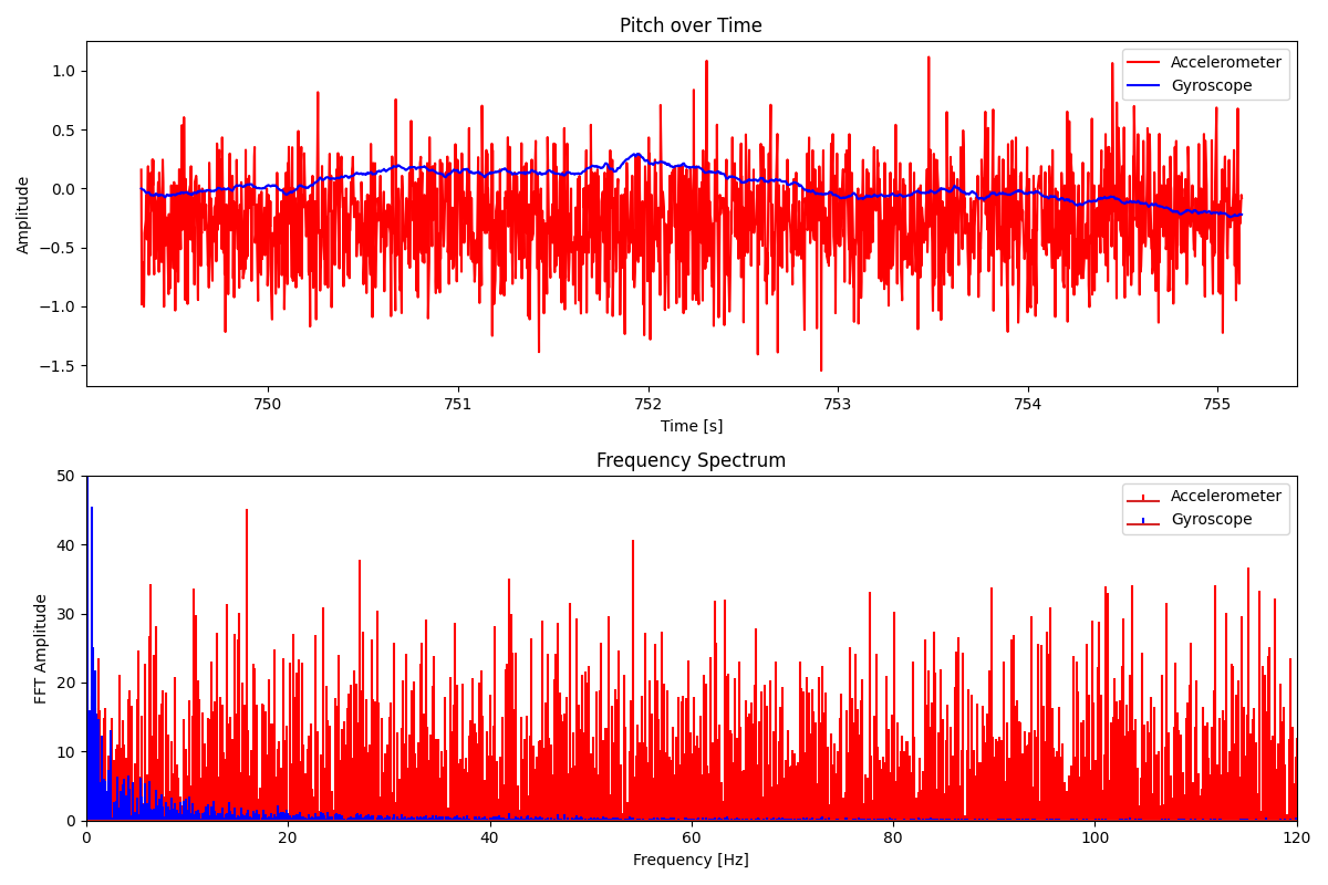
When the IMU is stationary, it can be seen the pitch and roll of the gyro scope matches that of the accelerometer pretty well. There is signifigantly less noise in the gyroscope reading, at the cost of some minor drifting. The FFTs shows that the noise is negligible when there is no movement.

When we add some wobbling to the IMU, the drift becomes more prevalent.

Sampling Frequency

As I decreased sampling frequency, changes in pitch, roll, and yaw become more eratic, and drift increased in severity. I want to have as high of a sampling frequency as possible by decreasing delays and speeding up the main loop.

Complementary Filter

This is the complementary filter equation that we discussed in class. \(\theta_c = (\theta_c + \theta_g)(1-\alpha)+\alpha \theta_a\)

The idea of this filter is that each successive sample is a weighted mean of the gyroscope and accelerometer measurement.

roll_c_array[i] = (roll_c_array[i - 1] + (gX * dt)) * (1 - alpha) + roll_array[i] * alpha;
pitch_c_array[i] = (pitch_c_array[i - 1] + (-gY *dt)) * (1 - alpha) + (pitch_array[i] * alpha);

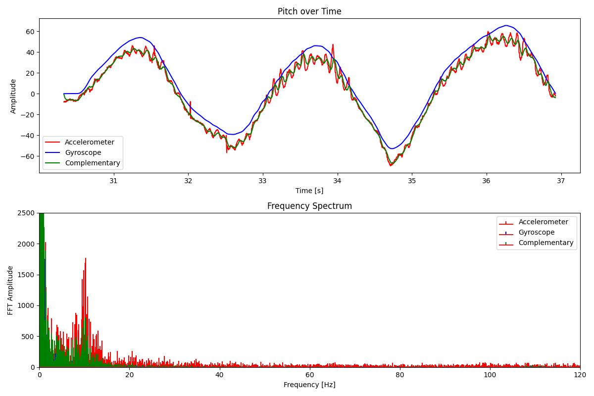
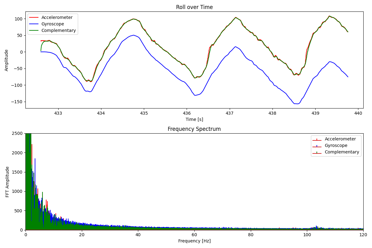
For the pitch measurement, I wobbled the IMU up and down shakily. Unsurprisingly, the accelerometer data is very noisy, and the gyroscope data drifts downwards. However, the complementary filter takes both into account and gives a reasonable signal free from quick vibration and drift. Since the complementary filter results run closer to the accelerometer data, it is not as free from noise as the gyroscope. The roll measurements show similar results, with less overall noise because I did not shake my hand during measurement.

Sample Data

Speed Up Execution

I took the following steps to speed up execution of the main loop

• IMU is only sampled when it signals that the data is ready. Otherwise, it just keeps looping unless the data is ready.
• Deleted all delay statements from the code. The blink on startup was changed to working without using delay().
• Removed all Serial.print() and Serial.println() statements.
• Send data point in batches instead of individually. Amount of data points in each batch depends on how many chars are needed to represent the data.
• My program is able to sample new values at about 400 samples per second.
• The main loop runs faster than the IMU can sample new values, but that is ok becuase sampling doesn’t occur unless the data is ready.

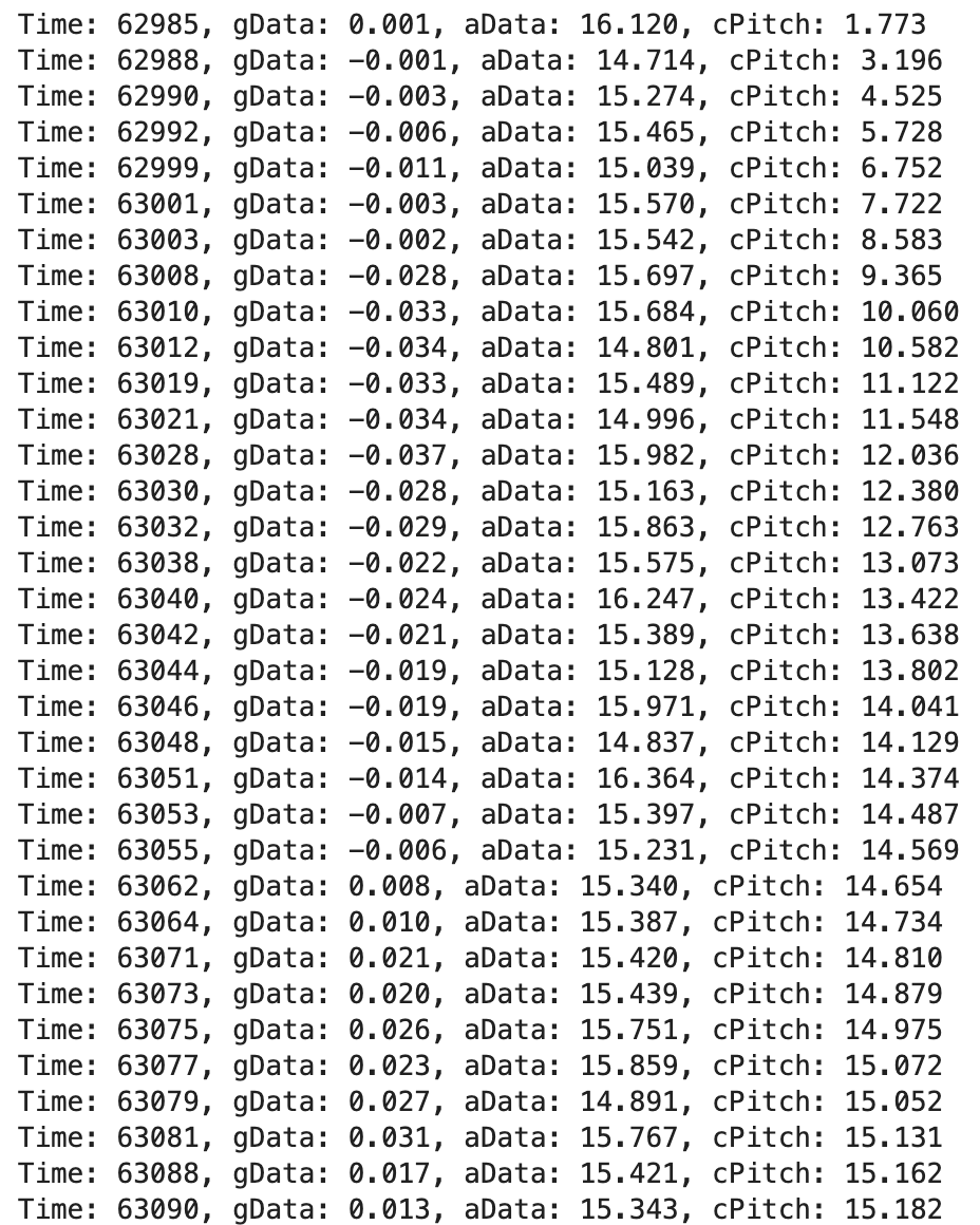
Time Stamped Data Points

Here is a screenshot of some time stamped data after it has been parsed by the notification handler, which is responsible for printing the data points, as well as appending them to arrays so they can be graphed with Matplotlib. A start and stop command can be sent to the board to tell it when to sample.

Data Storage

• For this lab, it makes more sense to store accelerometer and gyroscope data in seperate arrays. If I only want to send data from one type of sensor, having seperate arrays means that less data needs to be loaded into the cache. Additionally having seperate arrays makes the code easier to understand and maintain. The main advantage of having a single array is that data points from different sensors can be paired. By including timestamps with each measurement, synchronization can still be achieved using seperate arrays.
• Different data types should be used to store different types of data. For the time stamps, I am using the millis() command, which returns a whole number representing the amount of milliseconds that have passed since the start of the program. For time, there is no need to have sub-millisecond granularity, so it should be stored as an int. For data points such as pitch, roll, and yaw. I decided to use floats because high-frequency noise can have an amplitude of less than 0.5 degrees. Capturing this high frequency noise is important for determining a cutoff frequency for the filters.
• After uploading my program, the Artemis has 267904 bytes left for local variables. If each message is 151 chars (151 bytes), and each message can contain 3 data points, then my program can store nearly 600s of IMU data before memory overflow.

5 Seconds of Data Demo

Looking at the time domain graph, this demonstrates that at least 5 seconds of IMU data can be can be recorded and sent.

Recording a Stunt!

Observations

• Moderate velocity foward and backwards
• High foward and backwards acceleration
• Almost instant turning acceleration
• Very high turning velocity, hard to control
• Wheel is easy to break

References

• Worked with Jeffrey Cai to film stunts
• Used Mikayla Lahr Course Webpage for general report layout inspiration