Lab 11: Localization (real)

Prelab Testing

In this lab, I performed real localization using the Bayes filter. The filter was provided to me in the lab code, so I did not need to implement it myself. I used the same robot code as lab 9 to get the two input arrays, distance and yaw for a complete rotation. Before I writing code for the Jupyter notebook to receive data from my robot, I tested the localization simulation. In the results of the simulation are shown below.

The green line represents the actual path of the simulated robot, while the blue line is the positional prediction using the Bayes filter. Overall, The prediction matches the actual path pretty well. I noticed that the prediction strays from the actual path a little bit during large turns, which is to be expected. The prediction corrected itself quickly as soon as the robot starts to move linearly after the turn. I included a video of this behavior.

Implement Observation Loop

The next task of the lab was to implement the observation loop involving the actual robot. This was done in the perform_observation_loop function. First, I used BLE commands to set the PID variables and start the mapping rotation.

ble.send_command(CMD.SET_PID_GAINS, "0.1|0|0.0")
        ble.send_command(CMD.START_MAPPING, "")

The duration of the mapping routine depends on the friction of the surface that the robot is rotating on, so I timed a few iterations of the rotation for an average of 15 seconds. To give the system some leeway, I added a delay of 20 seconds, using asyncio.run(asyncio.sleep(20)), to make sure data isn’t requested before the mapping has finished. Using async.run allows me to avoid changing functions to async. I used my SEND_DATA command from lab 9 to request the distance and yaw array. Sending the data also takes time, so I check the length of the arrays at 3 second intervals to see if all the data has been received. No modifications were made to the Arduino code. Upon a successful transmission, I reshape the arrays into the proper form and return the results. The full function is shown below.

def perform_observation_loop(self, rot_vel=120):
    ble.send_command(CMD.SET_PID_GAINS, "0.1|0|0.0")
    ble.send_command(CMD.START_MAPPING, "")
    asyncio.run(asyncio.sleep(20))
    ble.send_command(CMD.SEND_DATA, "")

    while(len(tof1Arr) < 198 and len(yawArr) < 198):
        asyncio.run(asyncio.sleep(3))
        print(len(tof1Arr))


    rangeResult = np.array([x / 1000 for x in tof1Arr])
    
    # converting to column arrays
    rangeResult = np.array([x / 1000 for x in tof1Arr]).reshape(-1, 1)
    bearingResult = np.array(yawArr).reshape(-1, 1)

    # return results
    return rangeResult, bearingResult

Additionally, the update step depends on a uniform prior, so I implemented the get_pose function to return the starting position of the robot when it runs the observation loop. I wrote each position of the robot as comments so that they could be uncommented depending on which point in the world I was testing in.

    def get_pose(self):
        return (5*0.3048, -3*0.3048, 0), (5*0.3048, -3*0.3048, 0)
        #return (-5*0.3048, -3*0.3048, 0), (-5*0.3048, -3*0.3048, 0)
        #return (-2*0.3048, -3*0.3048, 0), (-2*0.3048, -3*0.3048, 0)
        #return (0, 3*0.3048, 0), (0, 3*0.3048, 0)
        #return (0, 0, 0), (0, 0, 0)

I was nearly ready to run the tests, but I realized that the notebook only supports 18 observations per position. My robot samples continuously without regard for robot orientation, so I had much more than 18 points. In fact, I had 199. I didn’t want to make changes to my robot code, so I found a way to increase the observations from 18 to 199 by editing the world.yaml file.

# Number of observations during the rotation behavior
# It is also the number of observations made in each discrete cell
# Must be an integer
observations_count: 199

That’s about it! I ran the update step of the localization at each of the marked points on the map. I included the mapping movement video from lab 9 because no changes were made to the physical robot or robot code.

Results

I tested the update step at the following points:

• (0, 0)
• (0, 3)
• (5, -3)
• (5, 3)
• (-2, -3)

All starting orientations were 0 degrees, facing the north side of the map.

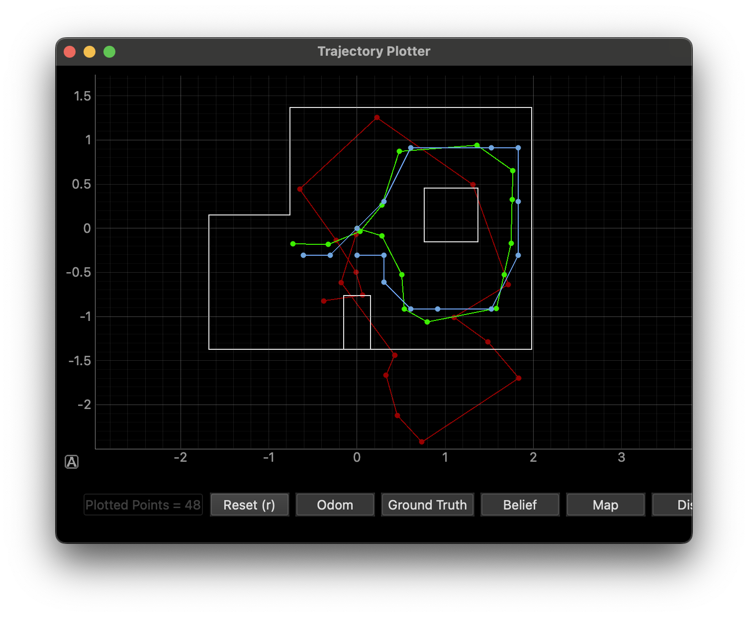
(0,0)

Localization at the origin was pretty accurate. If we only sample at one point, the origin produces the best mapping of of the world, so it makes sense that the belief was accurate at this position. There is less than a foot of error for this belief.

(0,3)

The localization at (0, 3) was not as good as the origin. I think this is because the ToF sensors don’t perform as well in more constrained areas. Also, the sensors might have periodically, sensed the ground instead of the world walls, making it think it’s in a more constrained position than it actually is. There is about 2 feet of error in this belief.

(5,-3)

The same problems that impacted (0, 3) were present in (5, 3).

(5,3)

The localization at (5, -3) was especially bad. The sensors might have periodically sensed the ground instead of the world walls, making it think it’s in a more constrained position than it actually is. This made the Bayes filter think that the robot was surrounded by walls inside of the square because it sensed so much of the ground in the readings. There is about 2 feet of error in this belief.

(-2,-3)

The localization at (-2, -3) was decent, strengthening the theory that a more open mapping area leads to better, more accurate beliefs.

References

• Thanks to Professor Helbling for explaining the purpose of the get_pose function!